
You are currently browsing the category archive for the ‘Problem of the Week (POW)’ category.
Huh — no solutions to POW-13 came in! I guess I was surprised by that.
Ah well, that’s okay. The problem wasn’t exactly trivial; there are some fairly deep and interesting things going on in that problem that I’d like to share now. First off, let me say that the problem comes from The Unapologetic Mathematician, the blog written by John Armstrong, who posted the problem back in March this year. He in turn had gotten the problem from Noam Elkies, who kindly responded to some email I wrote and had some pretty insightful things to say.
In lieu of a reader solution, I’ll give John’s solution first, and then mine, and then touch on some of the things Noam related in his emails. But before we do so, let me paraphrase what John wrote at the end of his post:
Here’s a non-example. Pick
points
and so on up to
. Pick
points
,
,
, and so on up to
. In this case we have
blocking points at
,
, and so on by half-integers up to
. Of course this solution doesn’t count because the first
Here’s a picture of that scenario when 

Does this configuration remind you of anything? Did somebody say “Pappus’s theorem“? Good. Hold that thought please.
Okay, in the non-example the first 


John Armstrong writes: Basically, I took the non-example and imagined bending back the two lines to satisfy the collinearity (pair-of-lines = degenerate conic, so non-example is degenerate example). The obvious pair of curves to use is the two branches of a hyperbola. But hyperbolas can be hard to work with, so I decided to do a projective transformation to turn it into a parabola.
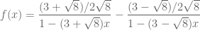
So let’s consider points on a parabola. The points  and
and  are connected by a line of slope
and are connected by a line of slope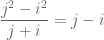
The line itself is 


Very nice. My own solution was less explicit in the sense that I didn’t actually write down coordinates of points, but gave instead a general recipe which relies instead on the geometry of conics, in fact on a generalization of Pappus’s theorem known to me as “Pascal’s mystic hexagon“. I first learned about this from a wonderful book:
- C. Herbert Clemens, A Scrapbook of Complex Curve Theory (2nd Edition), Graduate Studies in Mathematics 55, AMS (2002).
Pascal’s Mystic Hexagon, version A: Consider any hexagon inscribed in a conic, with vertices marked 


Pascal’s Mystic Hexagon, version B: Consider any pentagon inscribed in a conic 


The following solution uses version B.
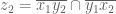
Solution by Todd and Vishal: For the sake of explicitness, let the conic 


To get started, notice that the blocking condition is trivially satisfied up to the point where we construct 


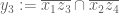
Suppose the blocking condition is satisfied for the points 


This shows that 


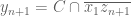
And so on up the inductive ladder: for 


Then, as prescribed above, we define 

What this argument shows (with Hexagon B doing all the heavy lifting) is that no cleverness whatsoever is required to construct the desired points: starting with any nondegenerate conic 
Which may lead one to ask: what is behind this “miracle” called Pascal’s Mystic Hexagon? Actually, not that much! Let me give a seat-of-the-pants argument for why one might expect it to hold, and then give a somewhat more respectable argument.
Define a planar cubic to be the locus 


has 10 coefficients. But the equation 


In the configuration for Pascal’s Mystic Hexagon, version A
we see three cubics passing through the 8 points 
where the conic


Since we expect that the space of cubics through these eight points is a line, we should have a linear relationship between the cubic polynomials 


for some scalars 


This rough argument isn’t too far removed from a slightly more rigorous one. There’s a general result in projective algebraic geometry called Bézout’s theorem, which says that a degree 


intersects the degree 2 conic 


for some degree 1 polynomial 

It’s clear then that what makes the Mystic Hexagon tick has something to do with the geometry of cubic curves. With that in mind, I’m now going to kick the discussion up a notch, and relate a third rather more sophisticated construction on cubics which basically subsumes the first two constructions. It has to do with so-called “elliptic curves“.
Officially, an elliptic curve is a smooth projective (irreducible) cubic “curve” over the complex numbers. I put “curve” in quotes because while it is defined by an equation 
Now a circle or 1-dimensional sphere 


if 

This is rather an interesting thing to prove, that this prescription actually satisfies the axioms for an abelian group. The hardest part is proving associativity, but this turns out to be not unlike what we did for Pascal’s Mystic Hexagon: basically it’s an application of Bézout’s theorem again. (In algebraic geometry texts, such as Hartshorne’s famous book, the discussion of this point can be far more sophisticated, largely because one can and does define elliptic curves as certain abstract 1-dimensional varieties or schemes which have no presupposed extrinsic embeddings as cubic curves in the plane, and there the goal is to understand the operations intrinsically.)
In the special case where 


Okay, here is a third solution to the problem, lifted from one of Noam Elkies’ emails. (The original formulation of the problem spoke in terms of 


“Choose points 


- red points:
,
- blue points:
,
- blocking points:
,


where 
Well, well. That’s awfully elegant. (According to Noam’s email, it came out of a three-way conversation between Roger Alperin, Joe Buhler, and Adam Chalcraft. Edit: Joe Buhler informs me in email that Joel Rosenberg’s name should be added. More at the end of this post.) Noam had given his own slick solution where again the red and blue points sit on a conic and the blocking points lie on a line not tangent to the conic, and he observed that his configuration was a degenerate cubic, leading him to surmise that his example could in a sense be seen as a special case of theirs.
How’s that? The last solution took place on a smooth (nondegenerate) cubic, so the degenerate cubic = conic+line examples could not, literally speaking, be special cases. Can the degenerate examples be seen in terms of algebraic group structures based on collinearity?
The answer is: yes! As you slide around in the space of planar cubics, nondegenerate cubics (the generic or typical case) can converge to cubics which are degenerate in varying degrees (including the case of three lines, or even a triple line), but the group laws on nondegenerate cubics based on collinearity converge to group laws, even in degenerate cases! (I hadn’t realized that.) You just have to be careful and throw away the singular points of the degenerate cubic, but otherwise you can basically still use the definition of the group law based on collineation, although it gets a little tricky saying exactly how you’re supposed to add points on a line component, such as the line of conic+line.
So let me give an example of how it works. It seems convenient for this purpose to use John Armstrong’s model which is based on the parabola+line, specifically the locus of 

We can maybe guess that since 

One is then led to consider that the group structure of this cubic overall is isomorphic to the group 


I claim that the abelian group structure on the punctured

so that the identity element on the cubic is 


Undoubtedly this group law looks a bit strange! So let’s do a spot check. Suppose 


is correct according to the group law, so the three collinear points do add to the identity and everything checks out.
All right, let’s retrieve John’s example as a special case. Take 


which was John’s solution.
Another long post from yours truly. I was sorry no solutions came from our readers, but if you’d like another problem to chew on, here’s a really neat one I saw just the other day. Feel free to discuss in comments!
Exercise: Given a point on a circle, show how to draw a tangent to the point using ruler only, no compass. Hint: use a mystic hexagon where two of the points are “infinitesimally close”.
Added July 25: As edited in above, Joel Rosenberg also had a hand in the elliptic curves solution, playing an instrumental role in establishing some of the conjectures, such as that 
It’s been an awfully long time since I’ve posted anything; time to finally break the silence.
This problem appeared elsewhere on the internet some months ago; some of you may have already seen it. I don’t want to say right away where I saw it, because there was some commentary which included some rough hints which I don’t want to give, but I’ll be sure to give credit when the solution is published. I’ll bet some of you will be able to find a solution, and will agree it’s quite cute. Here it is:
Given integers
, show that it is possible to construct a set of
points in the plane, let’s say
, so that no three points of the set are collinear, and for which there exist points
, all lying on a straight line, and arranged so that on the line between any
and any
, some
lies between them.
So no 


Please submit solutions to topological[dot]musings[At]gmail[dot]com by Friday, July 17, 11:59 pm (UTC); do not submit solutions in Comments. Everyone with a correct solution will be inducted into our Hall of Fame! We look forward to your response.
The solutions are in! This problem of the week was interesting for me: the usual pattern has been that I pose problems that I’ve solved myself at some point in the past, giving me a kind of “inside edge” on understanding the solutions that come in. But, as I said in POW-12, the difference this time is that the solution I knew of came from someone else (Arin Chaudhuri). What was interesting for me — and given the circumstances, it was probably inevitable — is that some of the solutions we received forced me to make contact with some mathematics I’d only heard about but never studied. Let me get to that in a minute.
Another interesting thing for me — speaking now with my category theorist’s hat on — is how utterly simple and conceptual Arin’s proof was! I was pleased to see that regular problem solver Philipp Lampe also spotted it. Wait for it…
Solution I by Philipp Lampe, University of Bonn: The answer is 8.
Among the eight neighbors of an arbitrary vertex, all colors of an admissible coloring must occur. Thus, 8 is an upper bound for the maximum number of colors one can use. We have to show that there is an admissible coloring with eight colors.
The vertices of the 8-dimensional cube may be represented by vectors 


Now let our “colors” be the 8 elements 


be the unique 

Now, if 

What I love about this solution it is how natural it is. I’ll say a little more about this in remarks below.
But I also learned a thing or two by studying the next solution. It relies on the theory of Hamming codes, with which I was not conversant. Up to some small edits, here is exactly what Sune Jakobsen submitted:
Solution II by Sune Jakobsen (first-year student), University of Copenhagen: Since each vertex only has 8 neighbors, the answer cannot be greater that 8.
Now we construct such a coloring with 8 colors. An 8-dimensional cube can be represented by the graph with vertices in 

It remains to show that no vertex is neighbor to two vertices of the same color. The Hamming distance between these two vertices is 2, thus the Hamming distance between the first 7 bits of two neighbors must be 1 or 2. If two neighbors had the same color
Remarks:
1. Let me give a little background to Sune’s solution. Mathematically, the Hamming code called “(7, 4)” is the image of injective linear map

given by the 
1101
1011
1000
0111
0100
0010
0001
The Hamming code is what is known as an “error-correcting code”. Imagine that you want to send a 4-bit message (each bit being a 0 or 1) down a transmission line, but that due to noise in the line, there is the possibility of a bit being flipped and the wrong message being received. What can you do to help ensure that the intended message is received?
The answer is to add some “parity check bits” to the message. In the code (7, 4), one adds in three parity checks, so that the transmitted message is 7 bits long. What one does is apply the matrix 
How does this work? By having the receiver apply a parity-check matrix 

1010101
0110011
0001111
In the first place, 

By the way, Sune reminded us that Hamming codes also came up in a post by Greg Muller over at The Everything Seminar, who used the existence of a Hamming code in every dimension 
2. Within minutes of posting the original problem, we received a message from David Eppstein, who reported that the solution of 8 colors is essentially contained in a paper he coauthored with T. Givaris (page 4); his solution is close in spirit to Sune’s.
Arin Chaudhuri also surmised the connection to Hamming codes, and mentions that the problem (in a slightly different formulation) originally came from a friend of a friend, who blogs about a number of related problems on this page. Presumably the author had things like error-correcting codes in mind.
3. Sune and David noted that their solutions generalize to show that on the 

This is very easy to see by adapting Philipp’s method. Indeed, for each 


4. We’re still not sure what the story is in other dimensions. If 


![a_n = 2^{\left[\log_2 n\right]}](https://s0.wp.com/latex.php?latex=a_n+%3D+2%5E%7B%5Cleft%5B%5Clog_2+n%5Cright%5D%7D&bg=ffffff&fg=545454&s=0&c=20201002)
![\left[x\right]](https://s0.wp.com/latex.php?latex=%5Cleft%5Bx%5Cright%5D&bg=ffffff&fg=545454&s=0&c=20201002)
Solved by Arin Chaudhuri, David Eppstein, Sune Jakobsen, and Philipp Lampe. Thanks to all those who wrote in!
Happy holidays, folks! And happy birthday to Topological Musings, which Vishal started just a little over a year ago — we’ve both had a really good time with it.
And in particular with the Problem of the Week series. Which, as we all know, doesn’t come out every week — but then again, to pinch a line from John Baez’s This Week’s Finds, we never said it would: only that each time a new problem comes out, it’s always the problem for that week! Anyway, we’ve been very gratified by the response and by the ingenious solutions we routinely receive — please keep ’em coming.
This problem comes courtesy of regular problem-solver Arin Chaudhuri and — I’ll freely admit — this one defeated me. I didn’t feel a bit bad though when Arin revealed his very elegant solution, and I’d like to see what our readers come up with. Here it is:
What is the maximum number of colors you could use to color the vertices of an 8-dimensional cube, so that starting from any vertex, each color occurs as the color of some neighbor of that vertex? (Call two vertices neighbors if they are the two endpoints of an edge of the cube.)
Arin, Vishal, and I would be interested and pleased if someone solved this problem for all dimensions
Please submit solutions to topological[dot]musings[At]gmail[dot]com by Friday, January 2, 2009, 11:59 pm (UTC); do not submit solutions in Comments. Everyone with a correct solution will be inducted into our Hall of Fame! We look forward to your response.
The solutions to POW-11 are in! Or make that solution, unless you also count your hosts’: only one reader responded. Perhaps everyone has been distracted by the upcoming US presidential election?!
Composite solution by Philipp Lampe, University of Bonn, and Todd and Vishal: We claim there are exactly two functions 

Clearly 


where in a few places we have invoked the simple lemma that 


Since 

Therefore, using the inductive hypothesis that 


From equation (1) we also have

Comparing equations (2) and (3), we infer 


For even 


and by arguing as we did above, we derive the two equations


where the second follows from the first by inductive hypothesis. Multiplying (4) through by 

Remarks:
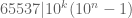
The underlying idea is to exploit the fact that many numbers can be expressed as a sum of two squares in more than one way, so that one can generate enough relations of the form 


![\mathbb{Z}\left[i\right]](https://s0.wp.com/latex.php?latex=%5Cmathbb%7BZ%7D%5Cleft%5Bi%5Cright%5D&bg=ffffff&fg=545454&s=0&c=20201002)

so that there are two ways of writing their product 65 in the form 

Here we have, respectively, 


then we have 

This gives a large supply of available relations to work with, and from there it is not too bad to get an inductive argument up and flying, once some base cases have been cleared out of the way with some numerical experimentation.
[Although it’s a little unusual to need such an outlay of base cases (up to at least 
Incidentally, while researching this problem, I found the wonderful website MathPages, created by an all but anonymous author named Kevin Brown. I really recommend checking out this website, and I hope that it is somehow kept alive: it would be a shame for such a treasure trove to be buried and forgotten in some deep hollow of cyberspace.
Time for another problem of the week! This one doesn’t necessarily require any number-theoretic knowledge, although a little bit might help point you in the right direction. As usual, let 
Describe all functions
.
Please submit solutions to topological[dot]musings[At]gmail[dot]com by Sunday, November 2, 11:59 pm (UTC); do not submit solutions in Comments. Everyone with a correct solution will be inducted into our Hall of Fame! We look forward to your response.
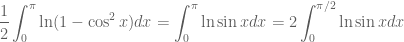
The solutions are in! As is so often the case, solvers came up with a number of different approaches; the one which follows broadly represents the type of solution that came up most often. I’ll mention some others in the remarks below, some of it connected with the lore of Richard Feynman.
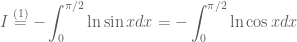
Solution by Nilay Vaish: The answer to POW-10 is 

and integrate by parts: we have

The first term vanishes by a simple application of L’hôpital’s rule. We now have
where the second equation follows from 


This gives

after a simple substitution. The last integral splits up as two integrals:
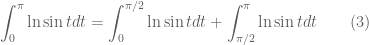
but these two integrals are equal, using the identity 
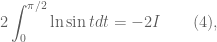
recalling equation (1) above. Substituting this for the last integral in equation (2), we arrive at

whence we derive the value of the desired integral 
Remarks:
1. A number of solvers exploited variations on the theme of the solution above, which could be summarized as involving symmetry considerations together with a double angle formula. For example, Philipp Lampe and Paul Shearer in their solutions made essential use of the identity

in conjunction with the complementarity 
2. Arin Chaudhuri (and Vishal in private email) pointed out to me that the evaluation of the integral

is actually fairly well-known: it appears for example in Complex Analysis by Ahlfors (3rd edition, p. 160) to illustrate contour integration of a complex analytic function via the calculus of residues, and no doubt occurs in any number of other places.
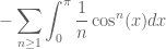
3. Indeed, Simon Tyler in his solution referred to this as an integral of Clausen type, and gave a clever method for evaluating it: we have

which works out to

The last integral can be expanded as a series
where the summands for odd
and by substituting this for the integral in (*), the original integral is easily evaluated.
4. Arin C. later described still another method which he says he got from an exercise in a book by Apostol — it’s close in spirit to the one I myself had in mind, called “differentiation under the integral sign”, famously referred to in Surely You’re Joking, Mr. Feynman!. As Feynman recounts, he never really learned fancy methods like complex contour integration, but he did pick up this method of differentiating under the integral sign from an old calculus book. In typical Feynman style, he writes,
“It turns out that’s not taught very much in the universities; they don’t emphasize it. But I caught on how to use that method, and I used that one damn tool again and again. So because I was self-taught using that book [Wilson’s Advanced Calculus], I had peculiar methods of doing integrals. The result was, when guys at MIT or Princeton had trouble doing a certain integral, it was because they couldn’t do it with the standard methods they had learned in school. If it was contour integration, they would have found it; if it was a simple series expansion, they would have found it. Then I come along and try differentiating under the integral sign, and often it worked. So I got a great reputation for doing integrals, only because my box of tools was different from everybody else’s, and they had tried all their tools on it before giving the problem to me.”
So, what is this method? Wikipedia has a pretty good article on it; the idea is to view a given definite integral 
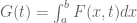


The best way to understand it is through an example. Pretend you’re Feynman, and someone hands you

[I suppose there may be a contour integration method to handle that one, but never mind — you’re Feynman now, and not supposed to know how to do that!] After fiddling around a little, you find that by inserting a parameter

this

i.e., by differentiating under the integral sign, you manage to kill off that annoying factor 

We therefore have
and notice that from the original definition of 


It takes a little experience to judge where or how to stick in the extra parameter

and I’ll let you the reader take it from there.
The point is not that this method is much more elegant than others, but that a little practice with it should be enough to convince one that it’s incredibly powerful, and often succeeds where other methods fail. (Not always, of course, and Feynman had to concede defeat when in response to a challenge, his pal Paul Olum concocted some hellacious integral which he said could only be done via contour integration.)
Doron Zeilberger is also fond of this method (as witnessed by this paper). Something about it makes me wonder whether it’s secretly connected with the idea of “creative telescoping” and the powerful methods (e.g., see here) developed by Gosper, Wilf, Zeilberger, and others to establish identities of hypergeometric type. But I haven’t had time to consider this carefully.
Also solved by Arin Chaudhuri, Philipp Lampe (University of Bonn), Paul Shearer (University of Michigan), and Simon Tyler. Thanks to all who wrote in!
Another problem of the week has been long overdue. Here’s one that may appeal to those who liked POW-5 (maybe we should have an integration problem every fifth time?):
Evaluate

Please submit solutions to topological[dot]musings[At]gmail[dot]com by Friday, October 10, 11:59 pm (UTC); do not submit solutions in Comments. Everyone with a correct solution will be inducted into our Hall of Fame! We look forward to your response.
It’s been quite a while since I’ve posted anything; I’ve been very busy with non-mathematical things this past month, and probably will be for at least another few weeks. In the meantime, I’d been idly thinking of another Problem of the Week to post, and while I was thinking of one such problem… I got stuck. So instead of just baldly posing the problem, this time I’ll explain how far as I got with it, and then ask you all for help.
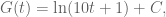
The problem is easy to state: except for 1, are there any positive integers which are simultaneously triangular, square, and pentagonal numbers?
Just asking for all numbers which are simultaneously triangular and square is a fun little exercise in number theory, involving Pell’s equation and (yes) continued fractions. I’ll sketch how this goes. We are trying to solve the Diophantine equation
By completing the square and manipulating a little, we get

This converts to a Pell equation 


and using the fact that the norm map 


forms a group, under the group multiplication law

which is read off just by expanding 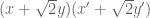

So, 

and in general, the solutions 

Let’s go back a minute to our original problem, which asked for numbers which are both triangular and square. We read off the 


and so the square 


It would be nice to express these solutions in closed form. To this end, let me observe that the quotients 


(A similar observation applies to any Pell equation: positive solutions to 


Starting from the first two rational approximants 


and for the purpose of determining the triangle-squares, we are really interested only in every other one of the denominators 


where the last equation follows easily from the recursive rule (*). The same recursion thus gives the 


namely 
To get a closed form for the

and use the recursive rule for the

The denominator expands as 
and from there, expanding the preceding line in geometric series, we derive a closed form for the
Nice! If you prefer, this is just the integer part of 
So, the

Sweet.
Having gone through this analysis, the same method can be used to determine those squares which are pentagonal (the first few pentagonal numbers are 

And that’s about as far as I got with this. After trying a few numerical forays with a hand-held calculator, my gut feeling is that I’d be amazed if there were any triangular-square-pentagonals past 
[Edit: I’ve corrected the exponents in the last displayed line, from 
The solutions are in! Last week’s POW-9 is a problem for which you need a bit of insight to solve at all (even with calculator or computer), and then a bit more to solve elegantly without machine aid.
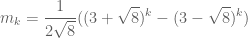
Solution by Philipp Lampe, University of Bonn: The answer is 


for integers 


Thus by minimality of 
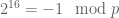
It is well known that 


Since 


(so that 

The second factor is, by the law of quadratic reciprocity (and the fact 
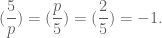
Also, by the “second supplement“, we compute 

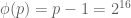
Remarks:The argument in the first paragraph of Philipp’s solution proves for 1/65537 a fact which holds generally for any reduced fraction 

A number of solvers computed the order of 10 by brute force, which I accepted. The use of quadratic reciprocity is slick but gets into rather deeper waters. As the Wikipedia article explains, this law was known to (or at least conjectured by) Euler and Legendre, but resisted a complete proof until Gauss found one after an intensive effort; it was one of his proudest achievements, and a theorem he returned to over the decades, giving over half a dozen more proofs in his life. Now more than 200 proofs are known. One proof that I like was given by Zolotarev, which is given a nice account in an appendix to John Conway’s very entertaining book, The (Sensual) Quadratic Form. Arin Chaudhuri pointed out to me that it’s also given as an exercise in Knuth’s The Art of Computer Programming (Vol. I, p. 45, exercise 47).
The “second supplement” was, according to the Wikipedia article, first proved by Euler. Its use here can be circumvented by observing that 2 cannot have order 

Quadratic reciprocity is no isolated curiosity: most of the deeper, more conceptual treatments involve some nontrivial algebraic number theory, and the efforts to formulate reciprocity laws for higher powers had a lot to do with the creation of class field theory, culminating in Artin reciprocity, one of the crowning achievements of early 20th century mathematics.
Also solved by Arin Chaudhuri, Ashwin Kumar, Vladimir Nesov, Américo Tavares, Nathan Williams, and Henry Wilton. Thanks to all who wrote in!


Recent Comments