Tag Archive

You are currently browsing the tag archive for the ‘Polya’ tag.

Inclusion-Exclusion Principle: Counting all the objects outside the oval regions!

March 20, 2008 in Exposition, Some theorems | Tags: inclusion-exclusion principle, Polya, Szego | by Vishal | 18 comments

Part 2:

After having understood the inclusion-exclusion principle by working out a few cases and examples in my earlier post, we are now ready to prove the general version of the principle.

As with many things in mathematics, there is a “normal” way of doing proofs and there is the “Polya/Szego” way of doing proofs. (Ok, ok, I admit it’s just a bias I have.) I will stick to the latter. Ok, let’s state the principle first and follow it up with its proof in a step-by-step fashion.

Inclusion-Exclusion Principle: Let there be a set of $N$ objects. Suppose out of these $N$ objects, there are $N_a$ objects of type $a$ , $N_b$ objects of type $b, \ldots ,$ $N_k$ objects of type $k$ and $N_l$ objects of type $l$ . Also, suppose $N_{ab}, N_{ac}, \ldots , N_{abc}, \ldots , N_{ab \ldots kl}$ denote the number of objects that are simultaneously of type $a$ AND $b,$ $a$ AND $c, \ldots , a, b$ AND $c, \ldots , a, b, c, k$ AND $l,$ respectively. Then, the number of objects that are NOT of type $a, b, c, \ldots , k, l$ is

$N - (N_a + N_b + \ldots + N_k + N_l)$

$+ (N_{ab} + N_{ac} + \ldots + N_{kl})$

$- (N_{abc} + \ldots ) + \ldots$

$\pm N_{abc \ldots kl}$ .

— Notation —

Let $U$ (finite or infinite) be the universe of discourse. Suppose $A \subset U$ . Then, the characteristic function $1_A: U \to \{ 0, 1 \}$ of $A$ is defined as

$1_A (x) = 1$ if $x \in A$ ,

and $1_A(x) = 0$ otherwise, for all $x \in U$ .

For example, suppose $U = \{ 1, 2, 3, 4, \ldots , 29, 30 \}$ . Let $A = \{ 2, 4, 6, \ldots , 28, 30 \}$ (i.e. even integers.) Then, $1_A(2) = 1_A(26) = 1, 1_A(3) = 1_A(29) = 0$ , and so on.

Note: $1_U (x) = 1$ and $1_{\emptyset}(x) = 0$ for all $x \in U$ . Here, $\emptyset$ denotes the empty set. Due to this, we will use $1$ and $1_U$ interchangeably from now.

—

Lemma 1: $A \subset B$ iff $1_A(x) \le 1_B(x)$ for all $x \in U$ .

Proof: We first prove the “only if”part. So, suppose $A \subset B$ . Let $x \in U$ . If $x \in A$ , then $1_A(x) = 1$ . But, we also have $x \in B$ , in which case, $1_B(x) = 1$ . If, on the other hand, $x \notin A$ , then $1_A(x) = 0 \le 1_B(x)$ . Hence, in either case, $1_A(x) \le 1_B(x)$ for all $x \in U$ .

We now prove the “if” part. So, suppose $1_A(x) \le 1_B(x)$ for all $x \in U$ . Let $x \in A$ . Then, $1_A(x) = 1$ , which forces $1_B(x) = 1$ , which implies $x \in B$ . Hence, $A \subset B$ , and this completes our proof.

Note: If $U$ is finite, then $\displaystyle |A| = \sum_{x \in U}1_A(x)$ .

Lemma 2: $1_{A^c}(x) = 1 - 1_A(x) ,$

$1_{A \cap B}(x) = 1_A(x) 1_B(x),$ and

$1_{A \cup B}(x) = 1 - (1 - 1_A(x))(1 - 1_B(x))$

for all $x \in U$ . (Here, $A^c$ is the complement of $A$ .)

Proof: The proof for each case is elementary.

Lemma 3: Suppose $U$ is finite. If $A, B, C, \ldots \subset U$ , then the characteristic function of $A \cup B \cup C \cup \ldots$ is $1 - (1 - 1_A)(1 - 1_B)(1 - 1_C) \ldots$ , i.e.

$1_{A \cup B \cup C \cup \ldots}(x) = 1 - (1 - 1_A(x))(1 - 1_B(x))(1 - 1_C(x)) \ldots$ for all $x \in U$ .

Proof: Note the above is an extension of the third part of lemma $(2)$ . A simple induction on the number of subsets of $U$ proves the result.

— Proof of the inclusion-exclusion principle —

Now, suppose $A, B, C, \ldots, K, L$ are subsets of objects of type $a, b, c, \ldots, k, l$ , respectively. Observe that the set of objects that are NOT of type $a, b, c, \ldots , k, l$ is simply the region outside of all the oval regions! (Look at the previous post to see what this means.) And this region is simply the subset $(A \cup B \cup B \cup \ldots \cup K \cup L)^c$ . Using the first part of lemma $(2)$ , we see that the characteristic function of this outside region is $1 - 1_{A \cup B \cup B \cup \ldots \cup K \cup L}$ , which from lemma $(3)$ is the same as

$(1-1_A)(1-1_B)(1-1_C) \ldots (1-1_K)(1-1_L)$ .

Expand the last expression to get

$1 - (1_A + 1_B + 1_C + \ldots)$

$+ (1_A1_B + 1_A1_C + \ldots)$

$- (1_A1_B1_C + \ldots) + \ldots$

$\pm 1_A1_B\ldots 1_L$ .

Now, sum over all the elements of $U$ and use the second part of lemma $(2)$ to obtain the desired result. And this completes our proof.

A Method of E. Landau (in complex analysis)

March 10, 2008 in Some theorems | Tags: e. landau, maximum modulus principle, Polya, Szego | by Vishal | 5 comments

[Update: Thanks to Andreas for pointing out that I may have been a little sloppy in stating the maximum modulus principle! The version below is an updated and correct one. Also, Andreas pointed out an excellent post on “amplification, arbitrage and the tensor power trick” (by Terry Tao) in which the “tricks” discussed are indeed very useful and far more powerful generalizations of the “method” of E. Landau discussed in this post. The Landau method mentioned here, it seems, is just one of the many examples of the “tensor power trick”.]

The maximum modulus principle states that if $f: U \to \mathbb{C}$ (where $U \subset \mathbb{C}$ ) is a holomorphic function, then $|f|$ attains its maximal value on any compact $K \subset U$ on the boundary $\partial K$ of $K$ . (If $|f|$ attains its maximal value anywhere in the interior of $K$ , then $f$ is a constant. However, we will not bother about this part of the theorem in this post.)

Problems and Theorems in Analysis II, by Polya and Szego, provides a short proof of the “inequality part” of the principle. The proof by E. Landau employs Cauchy’s integral formula, and the technique is very interesting and useful indeed. The proof is as follows.

From Cauchy’s integral formula, we have

$\displaystyle f(z) = \frac1{2\pi i} \oint_L \frac{f(\zeta)}{\zeta - z} d\zeta$ ,

for every $z$ in the interior of $D$ .

Now, suppose $|f(\zeta)| \le M$ on $L$ . Then,

$\displaystyle |f(z)| \le \frac{M}{2\pi} \int_L \left|\frac{d\zeta}{\zeta - z}\right| = KM$ ,

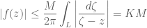
where the constant $K$ depends only on the curve $L$ and on the position of $z$ , and is independent of the specific choices of $f(z)$ . Now, this rough estimate can be significantly improved by applying the same argument to $(f(z))^n$ , where $n \in \mathbb{N}$ , to obtain

$|f(z)|^n \le K M^n$ , or $|f(z)| \le K^{1/n} M$ .

By allowing $n$ to go to infinity, we get $|f(z)| \le M$ , which is what we set out to prove.

Polya/Szego mention that the proof shows that a rough estimate may sometimes be transformed into a sharper estimate by making appropriate use of the generality for which the original estimate is valid.

I will follow this up with, maybe, a couple of problems/solutions to demonstrate the effectiveness of this useful technique.

Analysis/comments: an inequality problem in The HCMR, Issue 1 (2007)

December 23, 2007 in Problem Corner | Tags: AM-GM-HM inequality, Generalized Cauchy Inequality, Harvard College Mathematics Review, Inequality, Polya, Szego | by Vishal | 5 comments

The Harvard College Mathematics Review (HCMR) published its inaugural issue in April 2007, and the second issue was out almost a fortnight ago. Clearly, the level of exposition contained in the articles is extremely high, and it is a pleasure reading all the articles even though a lot of it may not make a lot of sense to a lot of people. I would recommend anyone to visit their website and browse all their issues. For problem-solvers, the problem section in each issue is a delight!

Anyway, the first issue’s problem section contained a somewhat hard inequality problem (proposed by Shrenik Shah), which I was able to solve and for which my solution was acknowledged in the problem section of the second issue. The HCMR carried Greg Price’s solution to that particular problem, and I must say his solution is somewhat more “natural” and “intuitive” than the one I gave.

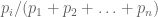
Well, I want to present my solution here but in a more detailed fashion. In particular, I want to develop the familiar $AM-GM-HM$ inequality up to a point where the solution to the aforesaid problem turns out to be somewhat “trivial.” The buildup to the final solution itself is non-trivial, however. This post relies on the material presented in the classic book Problems and Theorems in Analysis I by George Pólya and Gabor Szegö. Again, I strongly recommend all problem-solvers to study this book. Anyway, we will now state the problem and discuss its solution. (I have slightly changed the formulation of the problem in order to avoid any possible copyright issues.)

Problem: For all distinct positive reals $a$ and $b$ , show that

$\displaystyle \frac{a+b}{2} > \frac{a^{\frac{a}{a-b}}b^{\frac{b}{b-a}}}{e} > \frac{a-b}{\ln a - \ln b}$ .

First, let us discuss some facts.

1. $AM-GM-HM$ inequality: If $x_1, x_2, \ldots, x_n$ are $n$ positive real numbers, then

$\displaystyle (x_1 + x_2 + \ldots + x_n)/n \geq \sqrt[n]{x_1x_2\cdots x_n} \geq \frac{n}{1/x_1 + 1/x_2 + \ldots + 1/x_n}$ ,

with equality if and only if $x_1 = x_2 = \ldots = x_n$ .

Proof: For a hint on proving the above using mathematical induction, read this. However, we will make use of Jensen’s inequality to prove the above result. We won’t prove Jensen’s inequality here, though it too can be proved using induction.

Jensen’s inequality: Let $f : (a, b) \to \mathbb{R}$ be a continuous convex function. Let $\lambda_1, \lambda_2, \ldots, \lambda_n$ be positive reals such that $\lambda_1 + \lambda_2 + \ldots + \lambda_n = 1$ . Then for all $x_1, x_2, \ldots, x_n \in (a,b)$ , we have

$\lambda_1f(x_1) + \lambda_2f(x_2) + \ldots + \lambda_nf(x_n) \geq f(\lambda_1x_1 + \lambda_2x_2 + \ldots + \lambda_nx_n)$ ,

with equality if and only if $x_1 = x_2 = \ldots = x_n$ .

Now, in order to prove (1), consider the function $f : (0,\infty) \to \mathbb{R}$ defined by $f(x) = -\ln x$ . Indeed, $f$ is continuous on the stated domain. Also, $f''(x) = 1/x^2 > 0$ , which implies $f$ is convex on $(0, \infty)$ . Therefore, using Jensen’s inequality and setting $\lambda_1 = \lambda_2 = \ldots = \lambda_n = 1/n$ , for positive reals $x_1, x_2, \ldots, x_n$ , we have

$\displaystyle -\frac1{n} \left( \ln x_1 + \ln x_2 + \ldots + \ln x_n \right) \geq -\ln \left( \frac{x_1 + x_2 + \ldots + x_n}{n} \right)$

$\displaystyle \Rightarrow \frac{x_1 + x_2 + \ldots + x_n}{n} \geq \sqrt[n]{x_1x_2\cdots x_n} \quad \ldots$ (since $\ln x$ is monotonically increasing on $(0, \infty)$ .)

This proves the first part of the inequality in (1). Now, replace each $x_i$ with $1/x_i$ for $1 \leq i \leq n$ to derive the second part of the inequality. And, this proves the $AM-GM-HM$ inequality.

We can generalize this further. Indeed, for any positive reals $p_1, p_2, \ldots, p_n$ and positive reals $x_1, x_2, \ldots, x_n$ , replacing each $\lambda_i$ with $p_i/(p_1 + p_2 + \ldots + p_n)$ for $1 \leq i \leq n$ , and using Jensen’s inequality for $f(x) = -\ln x$ once again, we obtain the following generalized $AM-GM-HM$ inequality, which we shall call by a different name:

2. Generalized Cauchy Inequality (non-integral version) : For any positive reals $p_1, p_2, \ldots, p_n$ and positive reals $x_1, x_2, \ldots, x_n$ , we have

$\displaystyle \frac{p_1x_1 + \ldots + p_nx_n}{p_1 + \ldots + p_n} \geq \left( x_1^{p_1}\cdots x_n^{p_n}\right)^{1/(p_1 + \ldots + p_n)} \geq \frac{p_1 + \ldots + p_n}{p_1/x_1 + \ldots + p_n/x_n}$ .

Now, the remarkable thing is we can generalize the above inequality even further to obtain the following integral version of the inequality.

3. Generalized Cauchy Inequality (integral version) : Let $f(x)$ and $p(x)$ be continuous and positive functions on the interval [ $a, b$ ] ; also suppose $f(x)$ is not a constant function. Then we have

$\displaystyle \frac{\int_{a}^{b} p(x)f(x)\, dx}{\int_{a}^{b} p(x)\, dx} > \exp\left({\frac{\int_{a}^{b} p(x)\ln f(x)\, dx}{\int_{a}^{b} p(x)\, dx}}\right) > \frac{\int_{a}^{b} p(x)\, dx}{\int_{a}^{b} \frac{p(x)}{f(x)}\, dx}$ ,

where $\exp(x) = e^x$ .

Okay, now we are finally ready to solve our original problem. First, without any loss of generality, we can assume $a < b$ . Now, we shall use the above version of the Generalized Cauchy Inequality, and so we set $p(x) = 1$ and $f(x) = x$ . Here $f$ and $g$ are both positive functions on the interval [ $a, b$ ]. Also, note that $f$ is not a constant function.

Thus, we have $\displaystyle \frac{\int_a^b 1\, dx}{\int_a^b \frac1{x} \, dx} = \frac{a-b}{\ln a - \ln b} \quad \ldots (*)$ .

Also, $\exp \left( \frac{\int_a^b \ln x \, dx}{\int_a^b 1 \, dx} \right) = \exp \left( \frac{b\ln b - a\ln a - (b-a)}{b-a}\right) = \frac{a^{\frac{a}{a-b}} b^{\frac{b}{b-a}}}{e} \quad \ldots (**)$ .

And, $\displaystyle \frac{\int_a^b x\, dx}{\int_a^b 1 \, dx} = \frac{(b^2 - a^2)/2}{b-a} = \frac{a+b}{2} \quad \ldots (***)$ .

Combining $(*), (**)$ and $(***)$ , we immediately obtain the desired inequality. And, we are done.

	Strong equidistribut… on Platonic Solids and Euler…
	m.s.mohamed ansari on The 54th Carnival of Math…
	Convictions ·… on Continued fraction for e
	Wayne J. Mann on Solution to POW-12: A graph co…
	erneststephen on The 54th Carnival of Math…
	anhtraisg on p^q + q^p is prime
	prof dr drd horia or… on My first post
	prof drd horia orasa… on My first post
	prof dr mircea orasa… on Inequality with log
	notedscholar on Self-referential Paradoxes, In…
	prof dr mircea orasa… on Inequality with log
	prof dr mircea orasa… on Inequality with log
	prof dr mircea orasa… on 2010 in review
	kenji on Basic category theory, I
	prof dr mircea orasa… on Solution to POW-10: Another ha…

M	T	W	T	F	S	S
		1	2	3	4	5
6	7	8	9	10	11	12
13	14	15	16	17	18	19
20	21	22	23	24	25	26
27	28	29	30	31

Tag Archive

Inclusion-Exclusion Principle: Counting all the objects outside the oval regions!

A Method of E. Landau (in complex analysis)

Analysis/comments: an inequality problem in The HCMR, Issue 1 (2007)

Our other blog

Visitors to this blog

Blog Stats

Wikio Ranking

Current Online Readers

Recent Comments

Top Posts

Archives

Categories

Blogroll

chess

Computers and Technology

Elementary Math Problem Solving

Fun, Humor

Higher Mathematics

Math Education

Non-technical

Opinions

People in Computer Science

People in mathematics

Philosophy & Logic

Physics

Politics, News

Sciences

Useful general links

Useful Math Links

Tag Cloud

Admin/Users Login

Pages