Self-referential Paradoxes, Incompleteness and Fixed Points

Who doesn’t like self-referential paradoxes? There is something about them that appeals to all and sundry. And, there is also a certain air of mystery associated with them, but when people talk about such paradoxes in a non-technical fashion indiscriminately, especially when dealing with Gödel’s incompleteness theorem, then quite often it gets annoying!

Lawvere in ‘Diagonal Arguments and Cartesian Closed Categories‘ sought, among several things, to demystify the incompleteness theorem. To pique your interest, in a self-commentary on the above paper, he actually has quite a few harsh words, in a manner of speaking.

“The original aim of this article was to demystify the incompleteness theorem of Gödel and the truth-definition theory of Tarski by showing that both are consequences of some very simple algebra in the cartesian-closed setting. It was always hard for many to comprehend how Cantor’s mathematical theorem could be re-christened as a“paradox” by Russell and how Gödel’s theorem could be so often declared to be the most significant result of the 20th century. There was always the suspicion among scientists that such extra-mathematical publicity movements concealed an agenda for re-establishing belief as a substitute for science.”

In the aforesaid paper, Lawvere of course uses the language of category theory – the setting is that of cartesian closed categories – and therefore the technical presentation can easily get out of reach of most people’s heads – including myself. Thankfully, Noson S. Yanofsky has written a nice paper, ‘A Universal Approach to Self-Referential Paradoxes, Incompleteness and Fixed Points’, that is a lot more accessible and fun to read as well.Yanofsky employs only the notions of sets and functions, thereby avoiding the language of category theory, to bring out and make accessible as much as possible the content of Lawvere’s paper. Cantor’s theorem, Russell’s Paradox, the non-definability of satisfiability, Tarski’s non-definability of truth and Gödel’s (first) incompleteness theorem are all shown to be paradoxical phenomena that merely result from the existence of a cartesian closed category satisfying certain conditions. The idea is to use a single formalism to describe all these diverse phenomena.

(Dang, I just found that John Baez had already blogged on this before, way back in 2006!)

An Experiment in Cognitive Reasoning

Among several things, these days, I have been doing some (serious) reading of literature on psychology, cognitive development, learning, linguistics, philosophy and a few other subjects. Well, the ones I just named happen to be parts of interdisciplinary areas, which are precisely the ones I am interested in. Of course, on many levels those parts also have a lot to do with mathematics, especially mathematical education. Ok, that was just a little background I wanted to provide for the content of today’s post.

I need to do a small (online) experiment in order to test a hypothesis, which will be the subject of my next post. Let me not reveal too much for now. The experiment is in the form of two puzzles that I ask readers (you!) to solve. They are both “multiple choice” puzzles with exactly two correct answers to each. Please bear in mind that this is NOT an IQ test. It is also not meant to test how good you are at solving puzzles individually. I am really interested in “aggregate” results. That is, for testing my hypothesis, I am only interested in what the majority thinks are the right answers. What is more, you won’t be graded, and no one (not even me) will ever know if you got the right answers. Please submit answers to both the puzzles.

Lastly, please don’t cheat or try to look for answers offline or online. As I said, this is NOT a test!

Let us now look at the puzzles.

Puzzle 1:

There are four cards, labelled either X or Y on one side and either 3 or 7 on the other. They are laid out in a row with their top (visible) sides shown like this: X Y 3 7. A rule states: “If X is on one side then there must be a 3 on the other.” Which two cards do you need to turn over to find out if this rule is true?

1) X

2) Y

3) 3

4) 7

Puzzle 2:

As you walk into a bar, you see a large sign that reads, “To drink alcohol here you must be over 18.” There are four people in the bar. You know the ages of two of them, and can see what the other two are drinking. The situation is: Alisa is drinking beer; Dymphna is drinking Coke; Maureen is 30 years old; Lauren is 16 years old. Which two people would you need to talk to in order to check that the “over 18 rule” for drinking alcohol is being followed?

1) Alisa

2) Dymphna

3) Maureen

4) Lauren

If you think you have the answers to those puzzles, then please click here Puzzles to submit your answers. (I couldn’t use PollDaddy to embed the above puzzles in this post because I am not allowed more than 160 characters in a single question. What a pain!) So, please go ahead and click the above link to submit yours answers.

Note: I will keep this “poll” open for a week to collect as much data as possible. Thanks!

Update: It seems many readers weren’t aware of the short duration of the “poll” and that they would have very much liked to participate. So, I am extending the poll till Jan 7, 2010 for them.  (Doing so would also help me in collecting more data.)

Number of idempotent endofunctions

Last summer, Todd and I discussed a problem and its solution, and I had wondered if it was fit enough to be in the POW-series (on this blog) when he mentioned that the problem might be somewhat too easy for that purpose. Of course, I immediately saw that he was right. But, a few days back, I thought it wouldn’t be bad if we shared this cute problem and its solution over here, the motivation being that some of our readers may perhaps gain something out of it. What is more, an analysis of an egf solution to the problem lends itself naturally to a discussion of combinatorial species. Todd will talk more about it in the second half of this post. Anyway, let’s begin.

PROBLEM: Suppose , where is a positive natural number. Find the number of endofunctions satisfying the idempotent property, i.e. .

It turns out that finding a solution to the above problem is equivalent to counting the number of forests with nodes and height at most , which I found here (click only if you wish to see the answer!) at the Online Encyclopedia of Integer Sequences. If you haven’t clicked on that link yet and wish to solve the problem on your own, then please stop reading beyond this point.

SOLUTION: There are two small (and related) observations that need to be made. And, both are easy ones.

Lemma 1: has at least one fixed point.

Proof: Pick any and let , where . Then, using the idempotent property, we have , which implies . Therefore, is a fixed point, and this proves our lemma.

Lemma 2: The elements in that are not fixed points are mapped to fixed points of .

Proof: Suppose is not a fixed point such that .  Then, using the idempotent property again, we immediately have , which implies , thereby establishing the fact that itself is a fixed point. Hence, (which is not a fixed point) is mapped to some fixed point of .

In both the lemmas above, the idempotent property “forces” everything.

Now, the solution is right before our eyes! Suppose has fixed points. Then there are ways of choosing them. And, each of the remaining elements of  that are not fixed points are to be mapped to any one of the fixed points. And, there are a total of ways of doing that. So, summing over all , our final answer is .

Exponential Generating Function and Introduction to Species

Hi; Todd here. Vishal asked whether I would discuss this problem from the point of view of exponential generating functions (or egf’s), and also from a categorical point of view, using the concept of species of structure, which gives the basis for a categorical or structural approach to generatingfunctionology.

I’ll probably need to write a new post of my own to do any sort of justice to these topics, but maybe I can whet the reader’s appetite by talking a little about the underlying philosophy, followed by a quick but possibly cryptic wrap-up which I could come back to later for illustrative purposes.

Enumerative combinatorics studies the problem of counting the number of combinatorial structures of some type on an -element set, such as the number of idempotent functions on that set, or the number of equivalence relations, and so on. A powerful idea in enumerative combinatorics is the idea of a generating function, where we study the series by rolling them into a single analytic function, such as

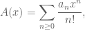
(this the so-called “exponential” generating function of ). In many cases of interest, the function will be recognizable in terms of operations familiar from calculus (addition, multiplication, differentiation, composition, etc.), and this can then be used to extract information about the series , such as explicit formulas, asymptotics, and so on. If you’ve never seen this idea in action, you should definitely take a look at Wilf’s book generatingfunctionology, or at the book Concrete Mathematics by Graham, Knuth and Patashnik.

Each of the basic operations one performs on analytic functions (addition, multiplication, composition, etc.) will, it turns out, correspond to some set-theoretic operation directly at the level of combinatorial structures, and one of the trade secrets of generating function technology is to have very clear pictures of the combinatorial structures being counted, and how these pictures are built up using these basic structural operations.

In fact, why don’t we start right now, and figure out what some of these structural operations would be? In other words, let’s ask ourselves: if and are generating functions for counting combinatorial structures of type (or species) and , then what types of structures would the function “count”?  How about ? Composition ?

The case of is easy: writing

and thinking of as counting structures of type on an -element set, and as counting structures of type , the quantity counts elements in the disjoint union of the sets of -structures and -structures.

In the categorical approach we will discuss later, we actually think of structure types (or species of structure) as functors, which take an -element set to the set of structures of type on . Here, we have to be a little bit careful about what categories we’re talking about, but the general idea is that if we have a bijection from one -element set to another, then it should always be possible to “transport” -structures on to -structures on , simply by relabeling points along the bijection . So, let us define a species to be a functor

where is the category of finite sets and bijections (not all functions, just bijections!), and is the category of sets. In enumerative combinatorics, the set is normally assumed to be finite, but in other applications of the notion of species, we actually allow a lot more latitude, and allow the functor to map into other categories , not just (“-valued species”). But if we stick for now just to set-valued species , , then we define the species by the functorial formula

where denotes disjoint union. So addition of generating functions will correspond to the concrete operation of taking disjoint unions of sets of combinatorial species.

More interesting is the case of multiplication. Let’s calculate the product of two egf’s:

The question is: what type of structure does the expression “count”? Look at the individual terms: the binomial coefficient describes the number of ways of decomposing an -element set into two disjoint subsets, one with elements and the other with , where and add to . Then, is the number of ways of putting an -structure on the -element part, and is the number of -structures on the -element part.

This suggests a new operation on structure types: given structure types or species , we define a new species according to the formula

(that is, a structure of type on a set is an ordered pair, consisting of an -structure on a subset of and a -structure on its complement). This functorial operation is usually called the “convolution product” of the combinatorial species : it is the concrete set-theoretic operation which corresponds to multiplication of generating functions.

Finally, let’s look at composition . Here we make the technical assumption that (no -structures on the empty set!), so that we won’t have divergence issues blowing up in our faces: we want to remain safely within the realm of finitary structures. Okay, then, what type of combinatorial structure does this egf count?

Perhaps not surprisingly, this is rather more challenging than the previous two examples. In analytic function language, we are trying here to give a meaning to the Taylor coefficients of a composite function in terms of the Taylor coefficients of the original functions — for this, there is a famous formula attributed to Faà di Bruno, which we then want to interpret combinatorially. If you don’t already know this but want to think about this on your own, then stop reading! But I’ll just give away the answer, and say no more for now about where it comes from, although there’s a good chance you can figure it out just by staring at it for a while, possibly with paper and pen in hand.

Definition: Let be species (functors from finite sets and bijections to finite sets), and assume . The substitution product is defined by the formula

This clearly requires some explanation. The sum here denotes disjoint union, and denotes the set of equivalence relations on the finite set . So here is an equivalence relation, which partitions into nonempty sets (-equivalence classes). And the quotient denotes the set of such equivalence classes (so we think of each class as a point of ). What this formula says is that a structure of type on consists of a partition of into a bunch of non-empty blobs, a -structure on each blob, and then an -structure on the set of blobs.

It’s high time for an example! So let’s look at Vishal’s problem, and see if we can picture it in terms of these operations. We’re going to need some basic functions (or functors!) to apply these operations to, and out of thin air I’ll pluck the two basic ones we’ll need:

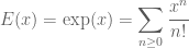
The first is the generating function for the series . So for the species , there’s just one structure of type for each set (in categorical language, the functor is the terminal functor). We can just think of that structure as the set itself, if we like, with no other structure appended thereon.

For , we have unless , where . So is the species for the one-element set structure (meaning that unless has cardinality 1, in which case ).

Okay, on to Vishal’s example. He was counting the number of idempotent functions , and now, as promised, I want to determine the corresponding egf. You might be able to find it by looking at his formula, but obviously I want to use the ideas I’ve developed thus far, which focuses much more on the pictures. So, let’s picture , first as Vishal did, by thinking of the elements of as ‘nodes’, and then drawing a directed edge from node to node if . (Then, by idempotence of , will be a fixed point of . Let’s agree not to bother drawing an edge from to itself, if is already a fixed point.)

In this picture, we get a directed graph which consists of a disjoint union of “sprouts”: little bushes, each rooted at a fixed point of , whose only other nodes are “leaves” joined to the root by an edge. We can simplify the picture a little: if you put a circle around each sprout, you don’t need the edges at all: just mark one of the points inside as the root, and you know what to do.

So we arrive at a picture of an idempotent function on : a partition of into a collection of (nonempty) blobs, and inside each blob, one of the points is marked “root”. In terms of our operations, what does it mean to mark a point in a blob? It just means: break the blob into two pieces, where one piece is given the structure of “one-element set”, and the other piece is just itself. In terms of the ideas developed above, this means each blob carries a structure; we’ll suggestively write this structure type as .

In this picture of idempotent , there is no extra combinatorial structure imposed on the set of blobs, beyond the set itself. In other words, in this picture, the set of blobs carries merely an “-structure”, nothing more.

So, putting all this together, we picture an idempotent function on as a partition or equivalence relation on , together with an assignment of a marked point in each equivalence class. In the language of species operations, we may therefore identify the structure type of idempotent functions with

or more suggestively, . The exponential generating function is, of course, !

In summary, the theory of species is a functorial calculus which projects onto its better-known “shadow”, the functional calculus of generating functions. That is to say, we lift operations on enumeration sequences , as embodied in their generating functions, directly up to the level of the sets we’re counting, where the functorial operations become both richer and more concrete. The functorial analogue of the generating function itself is called the “analytic functor” attached to the species (the species itself being the concrete embodiment of the enumeration).

Much more could be said, of course. Instead, here’s a little exercise which can be solved by working through the ideas presented here: write down the egf for the number of ways a group of people can be split into pairs, and give an explicit formula for this number. Those of you who have studied quantum field theory may recognize this already (and certainly the egf is very suggestive!) ; in that case, you might find interesting the paper by Baez and Dolan, From Finite Sets to Feynman Diagrams, where the functorial point of view is used to shed light on, e.g., creation and annihilation operators in terms of simple combinatorial operations.

The literature on species (in all its guises) is enormous, but I’d strongly recommend reading the original paper on the subject:

• André Joyal, Une théorie combinatoire des séries formelles, Adv. Math. 42 (1981), 1-82.

which I’ve actually referred to before, in connection with a POW whose solution involves counting tree structures. Joyal could be considered to be a founding father of what I would call the “Montreal school of combinatorics”, of which a fine representative text would be

• F. Bergeron, G. Labelle, and P. Leroux, Combinatorial Species and Tree-like Structures, Encyclopedia of Mathematics and its Applications 67, 1998.

More to come, I hope!

A Mathematical Chess (Dissection) Paradox

I thought I would share with our chess-loving readers the following interesting (and somewhat well-known) mathematical chess paradox , apparently proving that , and the accompanying explanation offered by Prof. Christian Hesse, University of Stuttgart (Germany).  It shows a curious connection between the well-known Cassini’s identity (related to Fibonacci numbers) and the chessboard ( being a Fibonacci number!). The connection can be exploited further to come up with similar paradoxes wherein any -square can always be “rerranged” to form a -rectangle such that the difference between their areas is either or . Of course, for the curious reader there are plenty of such dissection problems listed in Prof David Eppstein’s Dissection page.

Solution to POW-12: A graph coloring problem

The solutions are in! This problem of the week was interesting for me: the usual pattern has been that I pose problems that I’ve solved myself at some point in the past, giving me a kind of “inside edge” on understanding the solutions that come in. But, as I said in POW-12, the difference this time is that the solution I knew of came from someone else (Arin Chaudhuri). What was interesting for me — and given the circumstances, it was probably inevitable — is that some of the solutions we received forced me to make contact with some mathematics I’d only heard about but never studied. Let me get to that in a minute.

Another interesting thing for me — speaking now with my category theorist’s hat on — is how utterly simple and conceptual Arin’s proof was! I was pleased to see that regular problem solver Philipp Lampe also spotted it. Wait for it…

Solution I by Philipp Lampe, University of Bonn: The answer is 8.

Among the eight neighbors of an arbitrary vertex, all colors of an admissible coloring must occur. Thus, 8 is an upper bound for the maximum number of colors one can use. We have to show that there is an admissible coloring with eight colors.

The vertices of the 8-dimensional cube may be represented by vectors with in , in other words as vectors in , the 8-dimensional vector space over the field with two elements (i.e., the integers modulo 2). Two such vectors are neighbors iff their coordinate vectors differ in exactly one place, in other words if considered modulo 2, where is one of the eight standard basis elements (with -th coordinate 1, and the other coordinates 0).

Now let our “colors” be the 8 elements of , the 3-dimensional vector space over . Let the vertex “coloring”

be the unique -linear map such that ; that is, define the color of a vertex/vector by

Now, if is any vector, the colors of its neighbors are . The colors of these neighbors are all distinct since the are distinct. Hence all 8 colors are represented among the colors of the neighbors of any given vertex , QED.

What I love about this solution it is how natural it is. I’ll say a little more about this in remarks below.

But I also learned a thing or two by studying the next solution. It relies on the theory of Hamming codes, with which I was not conversant. Up to some small edits, here is exactly what Sune Jakobsen submitted:

Solution II by Sune Jakobsen (first-year student), University of Copenhagen: Since each vertex only has 8 neighbors, the answer cannot be greater that 8.

Now we construct such a coloring with 8 colors. An 8-dimensional cube can be represented by the graph with vertices in , and with an edge between them iff the Hamming distance between them is 1. We color a vertex with color 8 if the seven first bits in the vertex is a “correct” Hamming message (cf. Hamming code (7,4)), and color it in color if the first seven bits give a correct Hamming message upon changing bit . This is a well-defined coloring, since each element in is either a correct Hamming message, or is Hamming distance 1 away to exactly one correct Hamming message.

It remains to show that no vertex is neighbor to two vertices of the same color. The Hamming distance between these two vertices is 2, thus the Hamming distance between the first 7 bits of two neighbors must be 1 or 2. If two neighbors had the same color , then by definition one would get two correct Hamming messages by changing bit in both of them, and the Hamming distance between these messages would be the same as before — either 1 or 2. But the distance between any two correct Hamming messages is at least 3. Contradiction.

Remarks:

1. Let me give a little background to Sune’s solution. Mathematically, the Hamming code called “(7, 4)” is the image of injective linear map

given by the matrix

1101
1011
1000
0111
0100
0010
0001

The Hamming code is what is known as an “error-correcting code”. Imagine that you want to send a 4-bit message (each bit being a 0 or 1) down a transmission line, but that due to noise in the line, there is the possibility of a bit being flipped and the wrong message being received. What can you do to help ensure that the intended message is received?

The answer is to add some “parity check bits” to the message. In the code (7, 4), one adds in three parity checks, so that the transmitted message is 7 bits long. What one does is apply the matrix to the 4-vector, to get a 7-vector (remember we’re working modulo 2), and this 7-vector is sent down the line. Assuming only a moderate amount of noise in the transmission line, perhaps the 7-bit message will remain intact or perhaps a single bit will be flipped, more rarely two bits will be flipped (and we’ll assume the event that more than two are flipped has negligible probability). Now, the Hamming encoding is rigged up so that if the 7-bit vector is received as sent, then the parity checks will report 0 errors. If the parity checks report an error, they report precisely where the error occurred if the received vector was off by one bit. (If two flips occurred, then the receiver can still detect from the parity checks that an error occurred. The parity checks can never detect how many bits were flipped, but if the receiver assumes correctly that just one bit got flipped, he can restore the intended message with accuracy. If three or more got flipped, then the receiver got the wrong message, but he would never know it if the parity checks reported back 0 errors.)

How does this work? By having the receiver apply a parity-check matrix to the received message, given by the matrix

1010101
0110011
0001111

In the first place, , and so if the message received belongs to the image of (is a “correct Hamming message” in the terminology of Solution II), which will indeed be the case if there were no errors in the transmission, then applied to the message will produce the zero vector. In the case where one bit got flipped in the transmission, applied to the received vector will return a nonzero 3-vector, but the beauty of the Hamming code is that the 3-vector will spell out in binary the bit the error occurred (for example, if the output vector is , then error occurred in the bit with binary number 011, that is bit 3). In that case, the receiver flips that bit to restore the original message. In these two cases, the original 4 bits are then read off as the 3rd, 5th, 6th, and 7th coordinates of the (possibly corrected) 7-vector.

By the way, Sune reminded us that Hamming codes also came up in a post by Greg Muller over at The Everything Seminar, who used the existence of a Hamming code in every dimension to solve general hat-guessing puzzles.

2. Within minutes of posting the original problem, we received a message from David Eppstein, who reported that the solution of 8 colors is essentially contained in a paper he coauthored with T. Givaris (page 4); his solution is close in spirit to Sune’s.

Arin Chaudhuri also surmised the connection to Hamming codes, and mentions that the problem (in a slightly different formulation) originally came from a friend of a friend, who blogs about a number of related problems on this page. Presumably the author had things like error-correcting codes in mind.

3. Sune and David noted that their solutions generalize to show that on the -dimensional cube (for any ), it is possible to color the vertices with colors (the maximum number possible) so that all of the colors show up as colors of the neighbors of any given vertex.

This is very easy to see by adapting Philipp’s method. Indeed, for each just take the color set to be the -vector space . The set of vertices of the -dimensional cube may identified with the -vector space generated by the set (as basis), and the desired coloring is then just the -linear map that extends the identity function on . As mathematical constructions go, you can’t get much more canonical than that! No fuss, no muss — it’s a purely categorical construction (categorists call it a counit of an adjunction). So then why didn’t I see that myself? 🙂

4. We’re still not sure what the story is in other dimensions. If is the maximum number of admissible colors in dimension , then about all any one of us knows right now is that for , is weakly monotone increasing, and that if is not a power of 2. There’s a conjecture afloat that where is the floor function, but for now that should be treated as a wild guess. If anyone has further information, please let us know!

Solved by Arin Chaudhuri, David Eppstein, Sune Jakobsen, and Philipp Lampe. Thanks to all those who wrote in!

Using Mathematical Induction to “disprove” the foundation of Calculus!

Or, at least, that’s what this blog post at Science and Math Defeated aims to do. Normally, I avoid writing on such a topic but I think the following example could be instructive to a few people, at least, in learning how not to infer from mathematical induction. The author of that blog post sets to “disprove” the foundation of Calculus by showing that the “assumption” leads to a contradiction (which I am sure most of you have seen before.) And this is supposed to be achieved  through the use of Mathematical Induction.

Let be the statement for all  and .

Claim:  is true for all .

Proof: , and so,  is true. This takes care of the base case. Now assume  is true for some , where . Now, it is easy to show that  is true as well (I just skipped some details!). Hence,  holds. This takes care of the induction step. (Note that is shown to be true independent of !) And, this proves our claim.

(Erroneous) Conclusion: Hence, .

Notwithstanding the inductive proof (which is correct) above, why is the above conclusion wrong?

Ans. Because “infinity” is not a member of .

(Watch out for Todd’s next post in the ETCS series!)

POW-8: Ups at bat

Time for another Problem of the Week! This one is rather elementary, but is connected with a pet topic of mine which I plan to write a post on soon:

If a baseball player’s batting average is .334, what is the minimum number of times he’s been up at bat?

[Note for those who are not fans of baseball: a player’s batting average is (number of hits made)/(number of times at bat), rounded to three decimal places.]

Please submit solutions to topological[dot]musings[At]gmail[dot]com by Wednesday, July 30, 11:59 pm (UTC); do not submit solutions in Comments. Everyone with a correct solution will be inducted into our Hall of Fame! We look forward to your response.

Solution to POW-7: Midpoints between points on a curve

The solutions are in! There was quite a bit of activity behind the scenes on this one; POW-7 might look intuitively obvious, as if it should succumb to an easy application of the intermediate value theorem, but for a number of people who fought through it, this problem fought back! (And that was true for me too, when I first encountered it.)

This problem appears as problem B-4 from the 1977 Putnam Competition. A couple of readers hit upon the snappy solution proposed by the problem compilers [as given in The American Mathematical Monthly vol. 86 (1979), pp. 749-757]. I’ll give that solution, and follow up with a few remarks on alternate approaches, and on some of the thoughts the problem evoked in our readers. Thanks to all who wrote in!

Composite solution by Kenneth Chan and Paul Shearer: By translation, we may assume that the given point is the origin. Let . It suffices to show that is nonempty, for if belongs to this set, then both and , so that is the midpoint .

The interior regions of intersect (e.g., is in both regions), so if , then by connectedness of the curves , one of them must be contained in the interior of the other. But this is absurd; for example, it is clear that

and so if the sup is realized at a point which is interior to , then the boundary of the nonempty set contains a point of whose distance from the origin exceeds this shared sup, contradiction.

Remarks:

1. One could just as easily observe that the regions are congruent and therefore have the same area, so that one of these regions cannot be strictly contained in the other. Therefore, unless , some of is interior to and some is exterior; since is connected, it must therefore intersect the border of . Similarly, the exterior of must be partly inside and partly outside, so it too must intersect . In other words, some of is interior to and some is exterior to , and so by connectedness of , it must cross , as desired. This argument is substantially the one given by Sune Jakobsen.

2. Assuming is at the origin, a number of people tried to argue that (in polar coordinates) the radius of a point on is a function of its angle , and since sometimes takes non-positive values and sometimes non-negative values, it should take on the value 0 somewhere by the intermediate value theorem. The pitfall though is that is not necessarily a well-defined function of (consider non-convex curves where a radial line meets in more than one point). Some other readers seemed to notice this and tried a surrogate function where along the radial line at angle , you choose the closest distance from to the origin; the trouble there is that this new function might not be continuous (there will typically be a jump discontinuity at angles where the radial line is tangent to ).

3. The obstructions mentioned in remark 2. are of a sort which is ubiquitous in topology, where one would like to construct a continuous choice function (e.g., in the theory of vector bundles or fiber bundles, where one is interested in whether continuous sections of a bundle projection exist). À propos of that, Paul Shearer made an intriguing suggestion (in a comment here), that POW-7 would follow from the stronger conjecture that the space of pairs of points on which “straddle” (i.e., where the points and live on the same line, but the points are on opposite sides of ) should be path-connected. That is, given two pairs , the conjecture is that we can choose a continuous path through which gets us from to . Subsequently, Paul found a counterexample to this conjecture. Can you find one? [Edit: I had invited Paul to comment on this, but then missed the fact that he had already done so! My bad – TT.]

4. Miodrag Milenkovic came up with a related problem which can be posed in any dimension. Consider any -sphere embedded in (POW-7 concerns the case ), and let be a point interior to the embedded sphere. [Note: the complement of such an embedded sphere consists of two connected components, i.e., an “interior” and “exterior”, although this fact isn’t completely trivial; see theorem 36.3 (generalized Jordan curve theorem) in Munkres’s Elements of Algebraic Topology. These regions can be topologically complicated, as we know from the example of the Alexander horned sphere.] Miodrag asks: is it true that there exists a plane through so that is the center of mass (barycenter) of the -dimensional region where the interior intersects the plane?

I am not entirely decided on the answer to this question, although I think I have a nice topological argument that the answer is yes, if we assume some mild smoothness assumption on the embedding. I am frankly a little scared of the problem in full topological generality, due to the pathology one may encounter in the topological category!

POW-7 was also solved by Arin Chaudhuri, Sune Jakobsen, Philipp Lampe, and Peter LeFanu Lumsdaine. Thanks again to all for the stimulating correspondence!

POW-7: Midpoints between points on a curve

Okay, folks, time for another Problem of the Week! I hope it generates more response than last week’s problem:

Let be a simple closed curve in the plane, and let be any point strictly in the region interior to . Show there are two points on whose midpoint is .

Please submit solutions to topological[dot]musings[At]gmail[dot]com by Wednesday, July 9, 11:59 pm (UTC); do not submit solutions in Comments. Everyone with a correct solution will be inducted into our Hall of Fame! We look forward to your response.

POW-6: Tiling with Triominoes

This week’s problem is offered more in the spirit of a light and pleasant diversion — I don’t think you’ll need any deep insight to solve it. (A little persistence may come in handy though!)

Define a triomino to be a figure congruent to the union of three of the four unit squares in a square. For which pairs of positive integers is an rectangle tileable by triominoes?

Please submit solutions to topological[dot]musings[At]gmail[dot]com by Wednesday, July 3, 11:59 pm (UTC); do not submit solutions in Comments. Everyone with a correct solution will be inducted into our Hall of Fame! We look forward to your response. Enjoy!