
You are currently browsing the category archive for the ‘Boolean Algebra’ category.
After this brief (?) categorical interlude, I’d like to pick up the main thread again, and take a closer look at the some of the ingredients of baby Stone duality in the context of categorical algebra, specifically through the lens of adjoint functors. By passing a topological light through this lens, we will produce the spectrum of a Boolean algebra: a key construction of full-fledged Stone duality!
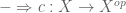
Just before the interlude, we were discussing some consequences of baby Stone duality. Taking it from the top, we recalled that there are canonical maps


in the categories of Boolean algebras 

What we have here is an adjoint pair of functors between the categories 


(


given by the formula 


The functor 
Earlier, we remarked that an ultrafilter in a Boolean algebra is a maximal filter, dual to a maximal ideal; let’s recall what that means. A maximal ideal 
i.e., has the form 


Conversely, a downward-closed subset 
we have that for all 


Thus we have redefined the notion of maximal ideal in a Boolean algebra in the first-order theory of posets: a downward-closed set 

The notion of ultrafilter is dual, so an ultrafilter in a Boolean algebra 
- Is upward-closed: if
and
;
- Is closed under finite meets: if
, then
;
- Satisfies dichotomy: for every
, exactly one of
belongs to
.
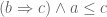
If 
Boolean algebra maps 

so that 
If 


maps 


We saw that when 

Proposition 1: If an ultrafilter
Proof: It is enough to show 


which contradicts the fact that 
It follows that nonprincipal ultrafilters can exist only on infinite sets
Proposition 2: Every (proper) filter in a Boolean algebra is contained in some ultrafilter.
Proof: This is dual to the statement that every proper ideal in a Boolean ring is contained in a maximal ideal. Either statement may be proved by appeal to Zorn’s lemma: the collection of filters which contain a given filter has the property that every linear chain of such filters has an upper bound (namely, the union of the chain), and so by Zorn there is a maximal such filter.
As usual, Zorn’s lemma is a kind of black box: it guarantees existence without giving a clue to an explicit construction. In fact, nonprincipal ultrafilters on sets
That said, one can still develop some intuition for ultrafilters. I think of them as something like “fat nets”. Each ultrafilter 


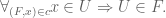
Intuitively speaking, ultrafilters as nets “move in a definite direction”, in the sense that given an element 


Since the intuitive imagery here is already vaguely topological, we may as well make the connection with topology more precise. So, suppose now that 

General topology can be completely developed in terms of the notion of ultrafilter convergence, often very efficiently. For example, starting with any relation whatsoever between ultrafilters and points,
we can naturally define a topology 
.
Let’s tackle that in stages: in order for the displayed condition to hold, a neighborhood of 
Then define a subset 
Proposition 3: This defines a topology,
Proof: Since 


Let’s recap: starting from a topology 


if and only if
Of course not every relation 

Theorem 1: If 


Proof: First I claim 


which in turn extends to some ultrafilter 
Corollary 1: Every filter is the intersection of all the ultrafilters which contain it.
The ultrafilter convergence approach to topology is particularly convenient for studies of compactness:
Theorem 2: A space
Proof: First suppose that 


In the reverse direction, suppose that every ultrafilter converges. We need to show that if 

Extend this filter to an ultrafilter 


Now let 


Conversely, suppose every ultrafilter converges to at most one point, and let 


Theorem 2 is very useful; among other things it paves the way for a clean and conceptual proof of Tychonoff’s theorem (that an arbitrary product of compact spaces is compact). For now we note that it says that a topology 
Here is our key example. Let 

where 


Chasing this a little further, the map 


This construction is about as “abstract nonsense” as it gets, but you have to admit that it’s pretty darned canonical! The topological space
It is first of all easy to see that 


you see immediately that 
To get Hausdorffness, take two distinct points 


Proposition 4: 
Proof: We must check that for all ultrafilters

But 
or that 

As a result, 


We actually get a lot more:
Proposition 5: The collection 
Proof: The sets 

between the two topologies. But a continuous bijection from a compact space to a Hausdorff space is necessarily a homeomorphism, so 
- Remark: In particular, the canonical topology on
is compact Hausdorff; this space is called the Stone-Cech compactification of (the discrete space)
is left adjoint to the underlying-set functor
. In fact, one can go rather further in this vein: a fascinating result (first proved by Eduardo Manes in his PhD thesis) is that the concept of compact Hausdorff space is algebraic (is monadic with respect to the monad
-ary operations (for each cardinal
, and whose models are precisely compact Hausdorff spaces. This goes beyond the scope of these lectures, but for the theory of monads, see the entertaining YouTube lectures by the Catsters!
Last time in this series on Stone duality, we observed a perfect duality between finite Boolean algebras and finite sets, which we called “baby Stone duality”:
- Every finite Boolean algebra
from
). The set
, the set of Boolean algebra homomorphisms from
- Conversely, every finite set
by taking its “hom-set”
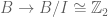
More precisely, there are natural isomorphisms


in the categories of finite Boolean algebras and of finite sets, respectively. In the language of category theory, this says that these categories are (equivalent to) one another’s opposite — something I’ve been meaning to explain in more detail, and I promise to get to that, soon! In any case, this duality says (among other things) that finite Boolean algebras, no matter how abstractly presented, can be represented concretely as power sets.
Today I’d like to apply this representation to free Boolean algebras (on finitely many generators). What is a free Boolean algebra? Again, the proper context for discussing this is category theory, but we can at least convey the idea: given a finite set 


First let me cut to the chase, and describe the key property of free Boolean algebras. Let 


To get a better grip on 


Idempotence also implies, as we saw last time, that 


where

i.e., the set of supports 

- Remark: This gives an algorithm for checking logical equivalence of two Boolean algebra formulas: convert the formulas into Boolean ring expressions, and using distributivity, idempotence, etc., write out these expressions as Boolean polynomials =
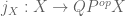
But there is another way of understanding free Boolean algebras, via baby Stone duality. Namely, we have the power set representation

where 


which takes a Boolean algebra map 


identifies each equivalence class of formulas 

- Remark: This is an instance of what is known as a completeness theorem in logic. On the syntactic side, we have a notion of provability of formulas (that
, or
in
. The method of truth tables then says that there are enough models or truth-value assignments to detect provability of formulas, i.e.,
There are still other ways of thinking about this. Let 
- The maximal ideal
in the Boolean ring
- The maximal filter or ultrafilter
in
Now, as we saw last time, in the case of finite Boolean algebras, each (maximal) ideal is principal: is of the form 

- A model of a finite Boolean algebra
Thus, baby Stone duality asserts a Boolean algebra isomorphism

Let’s give an example: consider the free Boolean algebra on three elements 


According to baby Stone duality, any element in the free Boolean algebra (with 

The unique expression of an element
All of the above applies not just to free (finite) Boolean algebras, but to general finite Boolean algebras. So, suppose you have a Boolean algebra 


The elements of 

In summary, any propositional theory (which by definition consists of a set 


Conversely, any Boolean algebra 

i.e., we may identify a model of a propositional theory with a Boolean algebra map 
So the set of models is the set

implies the following
Completeness theorem: If a formula of a finite propositional theory is “true” when interpreted under any model
Proof: Let ![b = [p] \in B](https://s0.wp.com/latex.php?latex=b+%3D+%5Bp%5D+%5Cin+B&bg=ffffff&fg=545454&s=0&c=20201002)


In summary, we have developed a rich vocabulary in which Boolean algebras are essentially the same things as propositional theories, and where models are in natural bijection with maximal ideals in the Boolean ring, or ultrafilters in the Boolean algebra, or [in the finite case] atoms in the Boolean algebra. But as we will soon see, ultrafilters have a significance far beyond their application in the realm of Boolean algebras; in particular, they crop up in general studies of topology and convergence. This is in fact a vital clue; the key point is that the set of models or ultrafilters
In this post, I’d like to move from abstract, general considerations of Boolean algebras to more concrete ones, by analyzing what happens in the finite case. A rather thorough analysis can be performed, and we will get our first taste of a simple categorical duality, the finite case of Stone duality which we call “baby Stone duality”.
Since I have just mentioned the “c-word” (categories), I should say that a strong need for some very basic category theory makes itself felt right about now. It is true that Marshall Stone stated his results before the language of categories was invented, but it’s also true (as Stone himself recognized, after categories were invented) that the most concise and compelling and convenient way of stating them is in the language of categories, and it would be crazy to deny ourselves that luxury.
I’ll begin with a relatively elementary but very useful fact discovered by Stone himself — in retrospect, it seems incredible that it was found only after decades of study of Boolean algebras. It says that Boolean algebras are essentially the same things as what are called Boolean rings:
Definition: A Boolean ring is a commutative ring (with identity 

Before I explain the equivalence between Boolean algebras and Boolean rings, let me tease out a few consequences of this definition.
Proposition 1: For every element 
Proof: By idempotence, we have 


This proposition implies that the underlying additive group of a Boolean ring is a vector space over the field 


Anyway, the point is that we can now apply some linear algebra to study this 


Now, the claim is that Boolean algebras and Boolean rings are essentially the same objects. Let me make this more precise: given a Boolean ring 

In one direction, suppose 


Notice also that 


Proposition 2: 
Proof: Looking at the definition of the order, this says that if 
So, 


or, replacing 

whence 
Proposition 3: 
Proof: We already saw 

using the formula for join we just computed. This completes the proof.
So the lattice is complemented; the only thing left to check is distributivity. Following the definitions, we have 

Naturally, we want to invert the process: starting with a Boolean algebra structure on a set 


after a short calculation using the complementation and distributivity axioms. After more work, one shows that
Exercise: Verify this last assertion.
However, the assertion of equivalence between Boolean rings and Boolean algebras has a little more to it: recall for example our earlier result that sup-lattices “are” inf-lattices, or that frames “are” complete Heyting algebras. Those results came with caveats: that while e.g. sup-lattices are extensionally the same as inf-lattices, their morphisms (i.e., structure-preserving maps) are different. That is to say, the category of sup-lattices cannot be considered “the same as” or equivalent to the category of inf-lattices, even if they have the same objects.
Whereas here, in asserting Boolean algebras “are” Boolean rings, we are making the stronger statement that the category of Boolean rings is the same as (is isomorphic to) the category of Boolean algebras. In one direction, given a ring homomorphism 


Theorem 1: The above processes define functors 

- Remark: I am taking some liberties here in assuming that the reader is already familiar with, or is willing to read up on, the basic notion of category, and of functor (= structure-preserving map between categories, preserving identity morphisms and composites of morphisms). I will be introducing other categorical concepts piece by piece as the need arises, in a sort of apprentice-like fashion.
Let us put this theorem to work. We have already observed that a finite Boolean ring (or Boolean algebra) has cardinality


Or, we can turn this around: for each 

Proposition 4: For a finite set 

Proof: We must show that for every Boolean ring map 


.
I claim that 


This proposition is a vital clue, for if 
With this in mind, our first claim is that there is a canonical Boolean ring homomorphism

which sends 


Theorem 2: If

is an isomorphism. (So, there is a natural isomorphism 
Proof: First we prove injectivity: suppose 


yields a homomorphism 

Now we prove surjectivity. A function 


(certainly 


Now let 


For the other direction, suppose 


from which it follows that 


- Remark: In proving both injectivity and surjectivity, we had in each case to pass back and forth between certain elements
for
whenever
(this second condition is equivalent to upward-closure:
implies
is a filter, by the De Morgan laws, and vice-versa. So via negation, there is a bijective correspondence between ideals and filters, and between maximal ideals and ultrafilters. Also, if
is a filter, just as the inverse image
is an ideal. Anyway, the point is that had we already had the language of filters, the proof of theorem 2 could have been written entirely in that language by straightforward dualization (and would have saved us a little time by not going back and forth with negation). In the sequel we will feel free to use the language of filters, when desired.
For those who know some category theory: what is really going on here is that we have a power set functor

(taking a function 


which we could replace by its opposite 


are components (at 


In this installment, I will introduce the concept of Boolean algebra, one of the main stars of this series, and relate it to concepts introduced in previous lectures (distributive lattice, Heyting algebra, and so on). Boolean algebra is the algebra of classical propositional calculus, and so has an abstract logical provenance; but one of our eventual goals is to show how any Boolean algebra can also be represented in concrete set-theoretic (or topological) terms, as part of a powerful categorical duality due to Stone.
There are lots of ways to define Boolean algebras. Some definitions were for a long time difficult conjectures (like the Robbins conjecture, established only in the last ten years or so with the help of computers) — testament to the richness of the concept. Here we’ll discuss just a few definitions. The first is a traditional one, and one which is pretty snappy:
A Boolean algebra is a distributive lattice in which every element has a complement.
(If 
- Example: Probably almost everyone reading this knows the archetypal example of a Boolean algebra: a power set
of a subset
and
.
- Example: Also well known is that the Boolean algebra axioms mirror the usual interactions between conjunction
, disjunction
, and negation
in ordinary classical logic. In particular, given a theory
, there is a preorder whose elements are sentences (closed formulas)
if the entailment
is provable in
iff
in
Exercise: Give an example of a complemented lattice which is not distributive.
As a possible leading hint for the previous exercise, here is a first order of business:
Proposition: In a distributive lattice, complements of elements are unique when they exist.
Proof: If both 


The definition of Boolean algebra we have just given underscores its self-dual nature, but we gain more insight by packaging it in a way which stresses adjoint relationships — Boolean algebras are the same things as special types of Heyting algebras (recall that a Heyting algebra is a lattice which admits an implication operator satisfying an adjoint relationship with the meet operator).
Theorem: A lattice is a Boolean algebra if and only if it is a Heyting algebra in which either of the following properties holds:
if and only if
for all elements

Proof: First let 


[Proof of claim: if 


In the other direction, given a lattice which satisfies 1., it is automatically a Heyting algebra (with implication 


On the other hand, suppose 


- Exercise: Show that Boolean algebras can also be characterized as meet-semilattices
.
The proof above invoked the De Morgan law 

Lemma: For any element 


Proof: First, we show that 


Corollary: 

- Remark: If we think of sups as sums and infs as products, then we can think of implications
as behaving like exponentials
. Indeed, our earlier result that
preserves infs
can then be recast in exponential notation as saying
, and our present corollary that
takes sups to infs can then be recast as saying
. Later we will state another exponential law for implication. It is correct to assume that this is no notational accident!
Let me reprise part of the lemma (in the case 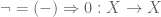
if and only if
if and only if
.
This situation is an instance of what is called a “Galois connection” in mathematics. If 


Here are some examples:
- The original example arises of course in Galois theory. If
is a field and
is a finite Galois extension with Galois group
(of field automorphisms
which fix the elements belonging to
and
. This works as follows: to each subset
, define
to be
. In the other direction, to each subset
, define
to be
. Both
and
are order-reversing (for example, the larger the subset
to belong to
iff (
for all
) iff
so we do get a Galois connection. It is moreover clear that for any
, and for any
- Another basic Galois connection arises in algebraic geometry, between subsets
(of a polynomial algebra over a field
. Given
(the zero locus of
. On the other hand, define
(the ideal of
. As in the case of Galois theory above, we clearly have a three-way equivalence
iff (
for all
) iff
so that
,
define a Galois connection between power sets (of the
). One defines an (affine algebraic) variety
are. Thus,
- Both of the examples above are particular cases of a very general construction. Let
be sets and let
be any relation between them. Then set up a Galois connection which in one direction takes a subset
, and in the other takes
to
. Once again we have a three-way equivalence
iff
iff
.
There are tons of examples of this flavor.


As indicated above, a Galois connection between posets 

Proposition:
- Given order-reversing maps
for all
for all
. (Given poset maps
which form an adjoint pair
, we have
for all
- Given a Galois connection as above,
for all
for all
induces a Galois correspondence between the elements of the form
and the elements of the form
.
Proof: (1.) It suffices to prove the statements for adjoint pairs. But under the assumption 
(2.) Again it suffices to prove the equations for the adjoint pair. Applying the order-preserving map
to 

Incidentally, the equations of 2. show why an algebraic variety 


Let 


Poset maps 


One virtue of closure operators is that they give a useful means of constructing new posets from old. Specifically, if 


One particular use is that the fixed points of the double negation closure 


The following exercises are in view of proving these results. If no one else does, I will probably give solutions next time or sometime soon.
Exercise: If 


Exercise: We have seen that 

Exercise: Show that double negation 
Exercise: If 

Exercise: Show that the fixed points of the double negation operator on a topology (as Heyting algebra) are the regular open sets, i.e., those open sets equal to the interior of their closure. Give some examples of non-regular open sets. Incidentally, is the lattice you get by taking the opposite of a topology also a Heyting algebra?


Recent Comments