
You are currently browsing the tag archive for the ‘topos theory’ tag.
After a long hiatus, I’d like to renew the discussion of axiomatic categorical set theory, more specifically the Elementary Theory of the Category of Sets (ETCS). Last time I blogged about this, I made some initial forays into “internalizing logic” in ETCS, and described in broad brushstrokes how to use that internal logic to derive a certain amount of the structure one associates with a category of sets. Today I’d like to begin applying some of the results obtained there to the problem of constructing colimits in a category satisfying the ETCS axioms (an ETCS category, for short).
(If you’re just joining us now, and you already know some of the jargon, an ETCS category is a well-pointed topos that satisfies the axiom of choice and with a natural numbers object. We are trying to build up some of the elementary theory of such categories from scratch, with a view toward foundations of mathematics.)
But let’s see — where were we? Since it’s been a while, I was tempted to review the philosophy behind this undertaking (why one would go to all the trouble of setting up a categories-based alternative to ZFC, when time-tested ZFC is able to express virtually all of present-day mathematics on the basis of a reasonably short list of axioms?). But in the interest of time and space, I’ll confine myself to a few remarks.
As we said, a chief difference between ZFC and ETCS resides in how ETCS treats the issue of membership. In ZFC, membership is a global binary relation: we can take any two “sets” 

Further, and far more radical: in ETCS the membership relation 


I believe it is reasonable to grant this principle a foundational status, but: rigorous adherence to this principle completely changes the face of what set theory looks like. If elements “belong” to only one set at a time, how then do we even define such basic concepts as subsets and intersections? These are some of these issues we discussed last time.
There are other significant differences between ZFC and ETCS: stylistically, or in terms of presentation, ZFC is more “top-down” and ETCS is more “bottom-up”. For example, in ZFC, one can pretty much define a subset 

But, in all fairness, that is perhaps the biggest obstacle to learning ETCS: at the outset, the tools available [mainly, the idea of a universal property] are quite simple but parsimonious, and one has to learn how to build some set-theoretic and logical concepts normally taken as “obvious” from the ground up. (Talk about “foundations”!) On the plus side, by building big logical machines from scratch, one gains a great deal of insight into the inner workings of logic, with a corresponding gain in precision and control and modularity when one would like to use these developments to design, say, automated deduction systems (where there tend to be strong advantages to using type-theoretic frameworks).
Enough philosophy for now; readers may refer to my earlier posts for more. Let’s get to work, shall we? Our last post was about the structure of (and relationships between) posets of subobjects 

Note to the experts: Most textbook treatments of the formal development of topos theory (as for example Mac Lane-Moerdijk) are efficient but highly technical, involving for instance the slice theorem for toposes and, in the construction of colimits, recourse to Beck’s theorem in monad theory applied to the double power-set monad [following the elegant construction of Paré]. The very abstract nature of this style of argumentation (which in the application of Beck’s theorem expresses ideas of fourth-order set theory and higher) is no doubt partly responsible for the somewhat fearsome reputation of topos theory.
In these notes I take a much less efficient but much more elementary approach, based on an arrangement of ideas which I hope can be seen as “natural” from the point of view of naive set theory. I learned of this approach from Myles Tierney, who was my PhD supervisor, and who with Bill Lawvere co-founded elementary topos theory, but I am not aware of any place where the details of this approach have been written up before now. I should also mention that the approach taken here is not as “purist” as many topos theorists might want; for example, here and there I take advantage of the strong extensionality axiom of ETCS to simplify some arguments.
The Empty Set and Two-Valued Logic
We begin with the easy observation that a terminal category, i.e., a category 

Let 
Proposition 0: If an ETCS category
Proof: Recall that a preorder is a category in which there is at most one morphism 


Assume from now on that
Proposition 1: There are at least two truth values, i.e., two elements 
Proof: By proposition 0, there exist sets 


Proposition 2: There are at most two truth values
Proof: If 


By propositions 1 and 2, there is a unique proper subset of the terminal object 


Proposition 3: 0 is an initial object, i.e., for any 
Proof: Uniqueness: if 


where 


Remark: For the “purists”, an alternative construction of the initial set 0 that avoids use of the strong extensionality axiom is to define the subset ![\left[\phi\right] \subseteq 1](https://s0.wp.com/latex.php?latex=%5Cleft%5B%5Cphi%5Cright%5D+%5Csubseteq+1&bg=ffffff&fg=545454&s=0&c=20201002)

where the first arrow represents the class of all subsets of 
Corollary 1: For any 
Proof: By cartesian closure, maps 

Corollary 2: If there exists 
Proof: The composite of 


By corollary 2, for any object 

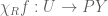
Proposition 4: If 
Proof: Under the assumption, 


External Unions and Internal Joins
One of the major goals in this post is to construct finite coproducts in an ETCS category. As in ordinary set theory, we will construct these as disjoint unions. This means we need to discuss unions first; as should be expected by now, in ETCS unions are considered locally, i.e., we take unions of subsets of a given set. So, let 
To define the union 


to the element 


Remark: Remember that in ETCS we are using generalized elements:
really means a function
over some domain
, which in turn classifies a subset
. On the other hand, the
. How then do we interpret the condition “
“? We first pull back
over to the domain
, and consider the condition that this is bounded above by
, thinking of the left side as constant over
.
We need to construct the subsets 
![A \subseteq \left[C\right]](https://s0.wp.com/latex.php?latex=A+%5Csubseteq+%5Cleft%5BC%5Cright%5D&bg=ffffff&fg=545454&s=0&c=20201002)

where the right side is the predicate “true over
Thus we construct the subset 

{C: A ≤ C} -------> 1
     |              |
     |              | t_X
     V chi_A => -   V
    PX -----------> PX
Let me take a moment to examine what this diagram means exactly. Last time we constructed an internal implication operator

and now, in the pullback diagram above, what we are implicitly doing is lifting this to an operator
The easy and cheap way of doing this is to remember the isomorphism 

to define 

Remark: Similarly we can define a meet operator
by exponentiating the internal meet
. It is important to know that the general Heyting algebra identities which we established last time for
on
, being a right adjoint, preserves products, and therefore preserves any algebraic identity which can be expressed as a commutative diagram of operations between such products.
Hence, for the fixed subset

classifies the subset

Finally, in the pullback diagram above, we are pulling back the operator 
we defined 


that one would expect “naively”.
Now that all the relevant constructions are in place, we show that
Here is a useful general principle for doing internal logic calculations. Let 


so that one has the general identity 


Lemma 1: Given a relation 


as subsets of
implies

as predicates over elements 
Proof: As we recalled above, 

Let

be the map which classifies the subset 
under the canonical isomorphisms 


Using the adjunction 

transforms to the composite

so by the pullback principle, 

Equivalently,

Also, as subsets of 

[this just says that 


Lemma 2: If 


Proof: From the last post, we have an adjunction:
if and only if

for any subset of 


where the first inclusion follows from 
Next, recall from the last post that the internal intersection of 

Lemma 3: If 
Proof: 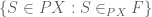


![\left[(S \in G) \Rightarrow (x \in S)\right] \leq \left[(S \in F) \Rightarrow (x \in S)\right]](https://s0.wp.com/latex.php?latex=%5Cleft%5B%28S+%5Cin+G%29+%5CRightarrow+%28x+%5Cin+S%29%5Cright%5D+%5Cleq+%5Cleft%5B%28S+%5Cin+F%29+%5CRightarrow+%28x+%5Cin+S%29%5Cright%5D&bg=ffffff&fg=545454&s=0&c=20201002)
Now apply lemma 2 to complete the proof.
Remark: The contravariance of
, that is, the fact that
implies
is a routine exercise using the adjunction [discussed last time]
if and only if
Indeed, we have
where the first inequality follows from the hypothesis
. By the adjunction, the inequality (*) implies
.


Theorem 1: For subsets 
Proof: It suffices to prove that 

to infer 

The condition we want,

is, by the adjunction 

which, by a 


as subsets of 

Using the adjunction 


which shows that the left side of (1) is contained in

where the last inclusion uses another
Now we prove the opposite inclusion
that is to say

Here we just use lemma 1, applied to the particular element
![\{x \in X: A \subseteq \left[\chi_A\right] \Rightarrow x \in_X A\}](https://s0.wp.com/latex.php?latex=%5C%7Bx+%5Cin+X%3A+A+%5Csubseteq+%5Cleft%5B%5Cchi_A%5Cright%5D+%5CRightarrow+x+%5Cin_X+A%5C%7D&bg=ffffff&fg=545454&s=0&c=20201002)
which collapses to 
![A = \left[\chi_A\right]](https://s0.wp.com/latex.php?latex=A+%3D+%5Cleft%5B%5Cchi_A%5Cright%5D&bg=ffffff&fg=545454&s=0&c=20201002)
Theorem 2: 


Proof: We are required to show that

Again, we just apply lemma 1 to the particular element 

but since 

which completes the proof.
Theorems 1 and 2 show that for any set

namely, the map which classifies the union of the subsets
![\displaystyle \left[\pi_1\right] = P1 \times 1 \stackrel{1 \times t}{\hookrightarrow} P1 \times P1](https://s0.wp.com/latex.php?latex=%5Cdisplaystyle+%5Cleft%5B%5Cpi_1%5Cright%5D+%3D+P1+%5Ctimes+1+%5Cstackrel%7B1+%5Ctimes+t%7D%7B%5Chookrightarrow%7D+P1+%5Ctimes+P1&bg=ffffff&fg=545454&s=0&c=20201002)
![\displaystyle \left[\pi_2\right] = 1 \times P1 \stackrel{t \times 1}{\hookrightarrow} P1 \times P1](https://s0.wp.com/latex.php?latex=%5Cdisplaystyle+%5Cleft%5B%5Cpi_2%5Cright%5D+%3D+1+%5Ctimes+P1+%5Cstackrel%7Bt+%5Ctimes+1%7D%7B%5Chookrightarrow%7D+P1+%5Ctimes+P1&bg=ffffff&fg=545454&s=0&c=20201002)
and this operation satisfies all the expected identities. In short,
We will come back to this point later, when we show (as a consequence of strong extensionality) that
Construction of Coproducts
Next, we construct coproducts just as we do in ordinary set theory: as disjoint unions. Letting

whose intersection is empty, and whose union or join in 


Theorem 3: A disjoint union of
Proof: It’s enough to embed 


is monic, one thus expects to be able to embed 
In detail, define 

where 


Clearly 


so it would be enough to show that each (or just one) of these two pullbacks is empty, let’s say the first.
Suppose given a map 
  A -------> 1
  |          |
h |          | chi_0
  V sigma_X  V
  X -------> PX
commute. Using the pullback principle, the map 

which is just the empty subset. This must be the same subset as classified by 

An elementary calculation shows this to be the equalizer of the pair of maps
So this equalizer 


Theorem 4: Any two disjoint unions of
Proof: Suppose 

where 


which is easily seen to be the diagonal on 


which is empty because 


Putting all this together, we conclude that 

Next, we show that 


If 


where 


The argument above shows that 


Theorem 5: The inclusions 

Proof: Let 


Now the operation 


exhibit 

whose restriction to 


I think that’s enough for one day. I will continue to explore the categorical structure and logic of ETCS next time.
This post is a continuation of the discussion of “the elementary theory of the category of sets” [ETCS] which we had begun last time, here and in the comments which followed. My thanks go to all who commented, for some useful feedback and thought-provoking questions.
Today I’ll describe some of the set-theoretic operations and “internal logic” of ETCS. I have a feeling that some people are going to love this, and some are going to hate it. My main worry is that it will leave some readers bewildered or exasperated, thinking that category theory has an amazing ability to make easy things difficult.
- An aside: has anyone out there seen the book Mathematics Made Difficult? It’s probably out of print by now, but I recommend checking it out if you ever run into it — it’s a kind of extended in-joke which pokes fun at category theory and abstract methods generally. Some category theorists I know take a dim view of this book; I for my part found certain passages hilarious, in some cases making me laugh out loud for five minutes straight. There are category-theory-based books and articles out there which cry out for parody!
In an attempt to nip my concerns in the bud, let me remind my readers that there are major differences between the way that standard set theories like ZFC treat membership and the way ETCS treats membership, and that differences at such a fundamental level are bound to propagate throughout the theoretical development, and impart a somewhat different character or feel between the theories. The differences may be summarized as follows:
- Membership in ZFC is a global relation between objects of the same type (sets).
- Membership in ETCS is a local relation between objects of different types (“generalized” elements or functions, and sets).
Part of what we meant by “local” is that an element per se is always considered relative to a particular set to which it belongs; strictly speaking, as per the discussion last time, the same element is never considered as belonging to two different sets. That is, in ETCS, an (ordinary) element of a set 


Instead, in ETCS, what we have is a local intersection operation on subsets 
Given two monomorphisms 


Taking some notational liberties, we write 


Thus, intersection works essentially the same way as in ZFC, only it’s local to subsets of a given set.
While we’re at it, let’s reformulate the power set axiom in this language: it says simply that for each set 


The equality is an equality between subsets, and the inverse image on the right is defined by a pullback. In categorical set theory notation,

Hence, there are natural bijections

between subsets and classifying maps. The subset corresponding to 
![\left[\phi\right] \subseteq B \times A](https://s0.wp.com/latex.php?latex=%5Cleft%5B%5Cphi%5Cright%5D+%5Csubseteq+B+%5Ctimes+A&bg=ffffff&fg=545454&s=0&c=20201002)
![\left[\phi\right] \subseteq A \times B](https://s0.wp.com/latex.php?latex=%5Cleft%5B%5Cphi%5Cright%5D+%5Csubseteq+A+%5Ctimes+B&bg=ffffff&fg=545454&s=0&c=20201002)
The set 

In ordinary set theory, the role of 


Lemma 1: The domain of elementhood 
Proof: A map 


Hence elementhood 


Part of the power of, well, power sets is in a certain dialectic between external operations on subsets and internal operations on

which maps an object 


- Remark: A category satisfying just the first three axioms of ETCS, namely existence of finite products, equalizers, and power objects, is called an (elementary) topos. Most or perhaps all of this post will use just those axioms, so we are really doing some elementary topos theory. As I was just saying, we can build up a tremendous amount of logic internally within a topos, but there’s a catch: this logic will be in general intuitionistic. One gets classical logic (including law of the excluded middle) if one assumes strong extensionality [where we get the definition of a well-pointed topos]. Topos theory has a somewhat fearsome reputation, unfortunately; I’m hoping these notes will help alleviate some of the sting.
To continue this train of thought: by the Yoneda lemma, the representing isomorphism

is determined by a universal element 
Internal Meets
To illustrate these ideas, let us consider intersection. Externally, the intersection operation is a natural transformation

This corresponds to a natural transformation

which (by Yoneda) is given by a function 


through the composite


Let’s analyze this bit by bit. The subset ![\left[\pi_1\right] = \pi_{1}^{-1}(t) \subseteq P(1) \times P(1)](https://s0.wp.com/latex.php?latex=%5Cleft%5B%5Cpi_1%5Cright%5D+%3D+%5Cpi_%7B1%7D%5E%7B-1%7D%28t%29+%5Csubseteq+P%281%29+%5Ctimes+P%281%29&bg=ffffff&fg=545454&s=0&c=20201002)

and the subset ![\left[\pi_2\right] = \pi_{2}^{-1}(t) \subseteq P(1) \times P(1)](https://s0.wp.com/latex.php?latex=%5Cleft%5B%5Cpi_2%5Cright%5D+%3D+%5Cpi_%7B2%7D%5E%7B-1%7D%28t%29+%5Csubseteq+P%281%29+%5Ctimes+P%281%29&bg=ffffff&fg=545454&s=0&c=20201002)

Hence ![\left[\pi_1\right] \cap \left[\pi_2\right] \subseteq P(1) \times P(1)](https://s0.wp.com/latex.php?latex=%5Cleft%5B%5Cpi_1%5Cright%5D+%5Ccap+%5Cleft%5B%5Cpi_2%5Cright%5D+%5Csubseteq+P%281%29+%5Ctimes+P%281%29&bg=ffffff&fg=545454&s=0&c=20201002)


The map 
To go from the internal meet 
if and only if

(where the equality signs are interpreted with the help of equalizers). This holds true iff 

A by-product of the interplay between the internal and external is that the internal intersection operator
is the meet operator of an internal meet-semilattice structure on 
if and only if

and this defines a reflexive, symmetric, antisymmetric relation ![\left[\leq\right] \subseteq P(1) \times P(1)](https://s0.wp.com/latex.php?latex=%5Cleft%5B%5Cleq%5Cright%5D+%5Csubseteq+P%281%29+%5Ctimes+P%281%29&bg=ffffff&fg=545454&s=0&c=20201002)
![\left[\leq\right] :=_i \{\langle u, v \rangle \in P(1) \times P(1): u = u \wedge v\},](https://s0.wp.com/latex.php?latex=%5Cleft%5B%5Cleq%5Cright%5D+%3A%3D_i+%5C%7B%5Clangle+u%2C+v+%5Crangle+%5Cin+P%281%29+%5Ctimes+P%281%29%3A+u+%3D+u+%5Cwedge+v%5C%7D%2C&bg=ffffff&fg=545454&s=0&c=20201002)
equivalently described as the equalizer
![\left[\leq\right] \to P(1) \times P(1) \stackrel{\to}{\to} P(1)](https://s0.wp.com/latex.php?latex=%5Cleft%5B%5Cleq%5Cright%5D+%5Cto+P%281%29+%5Ctimes+P%281%29+%5Cstackrel%7B%5Cto%7D%7B%5Cto%7D+P%281%29&bg=ffffff&fg=545454&s=0&c=20201002)
of the maps 
![\left[u\right] \subseteq \left[v\right]](https://s0.wp.com/latex.php?latex=%5Cleft%5Bu%5Cright%5D+%5Csubseteq+%5Cleft%5Bv%5Cright%5D&bg=ffffff&fg=545454&s=0&c=20201002)
Internal Implication
Here we begin to see some of the amazing power of the interplay between internal and external logical operations. We will prove that
Let’s recall the notion of Heyting algebra in ordinary naive set-theoretic terms: it’s a lattice 
if and only if

Now: by the universal property of 


Given 

(because

This means we should define
![\left[\leq\right] \subseteq P(1) \times P(1).](https://s0.wp.com/latex.php?latex=%5Cleft%5B%5Cleq%5Cright%5D+%5Csubseteq+P%281%29+%5Ctimes+P%281%29.&bg=ffffff&fg=545454&s=0&c=20201002)
Theorem 1:
Proof: We must check that for any three generalized elements 
if and only if

Passing to the external picture, let ![\left[u\right], \left[v\right], \left[w\right]](https://s0.wp.com/latex.php?latex=%5Cleft%5Bu%5Cright%5D%2C+%5Cleft%5Bv%5Cright%5D%2C+%5Cleft%5Bw%5Cright%5D&bg=ffffff&fg=545454&s=0&c=20201002)


![\left[u \Rightarrow v\right]](https://s0.wp.com/latex.php?latex=%5Cleft%5Bu+%5CRightarrow+v%5Cright%5D&bg=ffffff&fg=545454&s=0&c=20201002)

![e: \left[w\right] \to A](https://s0.wp.com/latex.php?latex=e%3A+%5Cleft%5Bw%5Cright%5D+%5Cto+A&bg=ffffff&fg=545454&s=0&c=20201002)
![\left[w\right] \subseteq A](https://s0.wp.com/latex.php?latex=%5Cleft%5Bw%5Cright%5D+%5Csubseteq+A&bg=ffffff&fg=545454&s=0&c=20201002)
Lemma 2: The composite
![\displaystyle u(e) = (\left[w\right] \stackrel{e}{\to} A \stackrel{u}{\to} P(1))](https://s0.wp.com/latex.php?latex=%5Cdisplaystyle+u%28e%29+%3D+%28%5Cleft%5Bw%5Cright%5D+%5Cstackrel%7Be%7D%7B%5Cto%7D+A+%5Cstackrel%7Bu%7D%7B%5Cto%7D+P%281%29%29&bg=ffffff&fg=545454&s=0&c=20201002)
is the classifying map of the subset ![\left[w\right] \cap \left[u\right] \subseteq \left[w\right]](https://s0.wp.com/latex.php?latex=%5Cleft%5Bw%5Cright%5D+%5Ccap+%5Cleft%5Bu%5Cright%5D+%5Csubseteq+%5Cleft%5Bw%5Cright%5D&bg=ffffff&fg=545454&s=0&c=20201002)
Proof: As subsets of ![\left[w\right]](https://s0.wp.com/latex.php?latex=%5Cleft%5Bw%5Cright%5D&bg=ffffff&fg=545454&s=0&c=20201002)
![(u e)^{-1}(t) = e^{-1} u^{-1}(t) = e^{-1}(\left[u\right]) = \left[w\right] \cap \left[u\right]](https://s0.wp.com/latex.php?latex=%28u+e%29%5E%7B-1%7D%28t%29+%3D+e%5E%7B-1%7D+u%5E%7B-1%7D%28t%29+%3D+e%5E%7B-1%7D%28%5Cleft%5Bu%5Cright%5D%29+%3D+%5Cleft%5Bw%5Cright%5D+%5Ccap+%5Cleft%5Bu%5Cright%5D&bg=ffffff&fg=545454&s=0&c=20201002)
![i: \left[u\right] \to A](https://s0.wp.com/latex.php?latex=i%3A+%5Cleft%5Bu%5Cright%5D+%5Cto+A&bg=ffffff&fg=545454&s=0&c=20201002)
Continuing the proof of theorem 1, we see by lemma 2 that the condition
![\left[w\right] \cap \left[u\right] \subseteq \left[w\right] \cap \left[v\right]](https://s0.wp.com/latex.php?latex=%5Cleft%5Bw%5Cright%5D+%5Ccap+%5Cleft%5Bu%5Cright%5D+%5Csubseteq+%5Cleft%5Bw%5Cright%5D+%5Ccap+%5Cleft%5Bv%5Cright%5D&bg=ffffff&fg=545454&s=0&c=20201002)
and this condition is equivalent to ![\left[w\right] \cap \left[u\right] \subseteq \left[v\right]](https://s0.wp.com/latex.php?latex=%5Cleft%5Bw%5Cright%5D+%5Ccap+%5Cleft%5Bu%5Cright%5D+%5Csubseteq+%5Cleft%5Bv%5Cright%5D&bg=ffffff&fg=545454&s=0&c=20201002)

Cartesian Closed Structure
Next we address a comment made by “James”, that a category satisfying the ETCS axioms is cartesian closed. As everything else in this article, this uses only the fact that such a category is a topos: has finite products, equalizers, and “power sets”.
Proposition 1: If 

Proof: By the power set axiom, there is a bijection between maps into the power set and relations:

which is natural in

Putting these together, we have a natural isomorphism

and this representability means precisely that 
Corollary 1: 
The universal element of this representation is an evaluation map 

Thus, 
As per our discussion, we want to internalize the set of such relations which are graphs of functions, i.e., maps 

where 

We see from this set-theoretic description that

which we can think of as either the equalizer of the pair of maps 

Thus, we put 


Now: a right adjoint such as 
       B^A ---------------> 1^A
        |                    |
sigma^A |                    | t^A
        V                    V
     P(B)^A -------------> P(1)^A
            (chi_sigma)^A
Of course, we don’t even have 


to the element in the hom-set (on the left) given by the composite

The map on the right of the pullback is defined similarly. That this recipe really gives a construction of
Universal Quantification
As further evidence of the power of the internal-external dialectic, we show how to internalize universal quantification.
As we are dealing here now with predicate logic, let’s begin by defining some terms as to be used in ETCS and topos theory:
- An ordinary predicate of type
. Alternatively, it is an ordinary element
. It corresponds (naturally and bijectively) to a subset
.
- A generalized predicate of type
. It may be identified with (corresponds naturally and bijectively to) a function
, or to a subset
.
We are trying to define an operator 


This function is determined by the subset 

Now, in ordinary logic, 


The expression on the right (global truth over 


Let’s check how this works externally. Let 

There is an interesting adjoint relationship between universal quantification and substitution (aka “pulling back”). By “substitution”, we mean that given any predicate 
![\psi(x) \wedge \left[a=a\right]](https://s0.wp.com/latex.php?latex=%5Cpsi%28x%29+%5Cwedge+%5Cleft%5Ba%3Da%5Cright%5D&bg=ffffff&fg=545454&s=0&c=20201002)
![(\left[\psi\right] \subseteq X) \mapsto (\left[\psi\right]\times A \subseteq X \times A).](https://s0.wp.com/latex.php?latex=%28%5Cleft%5B%5Cpsi%5Cright%5D+%5Csubseteq+X%29+%5Cmapsto+%28%5Cleft%5B%5Cpsi%5Cright%5D%5Ctimes+A+%5Csubseteq+X+%5Ctimes+A%29.&bg=ffffff&fg=545454&s=0&c=20201002)
Then, for any predicate
if and only if
![\left[\psi\right] \subseteq \forall_A \phi](https://s0.wp.com/latex.php?latex=%5Cleft%5B%5Cpsi%5Cright%5D+%5Csubseteq+%5Cforall_A+%5Cphi&bg=ffffff&fg=545454&s=0&c=20201002)
so that substitution along
Internal Intersection Operators
Now we put all of the above together, to define an internal intersection operator
which intuitively takes an element 
Let’s first write out a logical formula which expresses intersection:

We have all the ingredients to deal with the logical formula on the right: we have an implication operator 


There is a slight catch, in that the predicates “


and

Putting all this together, we form the composite


This composite directly expresses the definition of the internal predicate 


This construction provides an important bridge to getting the rest of the internal logic of ETCS. Since we can can construct the intersection of arbitrary definable families of subsets, the power sets 

As remarked above, the internal logic of a topos is generally intuitionistic (the law of excluded middle is not satisfied). But, if we add in the axiom of strong extensionality of ETCS, then we’re back to ordinary classical logic, where the law of excluded middle is satisfied, and where we just have the two truth values “true” and “false”. This means we will be able to reason in ETCS set theory just as we do in ordinary mathematics, taking just a bit of care with how we treat membership. The foregoing discussion gives indication that logical operations in categorical set theory work in ways familiar from naive set theory, and that basic set-theoretic constructions like intersection are well-grounded in ETCS.


Recent Comments