
You are currently browsing the category archive for the ‘Problem Corner’ category.
Last summer, Todd and I discussed a problem and its solution, and I had wondered if it was fit enough to be in the POW-series (on this blog) when he mentioned that the problem might be somewhat too easy for that purpose. Of course, I immediately saw that he was right. But, a few days back, I thought it wouldn’t be bad if we shared this cute problem and its solution over here, the motivation being that some of our readers may perhaps gain something out of it. What is more, an analysis of an egf solution to the problem lends itself naturally to a discussion of combinatorial species. Todd will talk more about it in the second half of this post. Anyway, let’s begin.
PROBLEM: Suppose
, where
is a positive natural number. Find the number of endofunctions
satisfying the idempotent property, i.e.
.
It turns out that finding a solution to the above problem is equivalent to counting the number of forests with 
SOLUTION: There are two small (and related) observations that need to be made. And, both are easy ones.
Lemma 1:
has at least one fixed point.
Proof: Pick any
and let
, where
. Then, using the idempotent property, we have
, which implies
. Therefore,
is a fixed point, and this proves our lemma.
Lemma 2: The elements in
that are not fixed points are mapped to fixed points of
Proof: Suppose
. Then, using the idempotent property again, we immediately have
, which implies
, thereby establishing the fact that
itself is a fixed point. Hence,
In both the lemmas above, the idempotent property “forces” everything.
Now, the solution is right before our eyes! Suppose
fixed points. Then there are
ways of choosing them. And, each of the remaining
elements of
ways of doing that. So, summing over all
.
Exponential Generating Function and Introduction to Species
Hi; Todd here. Vishal asked whether I would discuss this problem from the point of view of exponential generating functions (or egf’s), and also from a categorical point of view, using the concept of species of structure, which gives the basis for a categorical or structural approach to generatingfunctionology.
I’ll probably need to write a new post of my own to do any sort of justice to these topics, but maybe I can whet the reader’s appetite by talking a little about the underlying philosophy, followed by a quick but possibly cryptic wrap-up which I could come back to later for illustrative purposes.
Enumerative combinatorics studies the problem of counting the number 
(this the so-called “exponential” generating function of 

Each of the basic operations one performs on analytic functions (addition, multiplication, composition, etc.) will, it turns out, correspond to some set-theoretic operation directly at the level of combinatorial structures, and one of the trade secrets of generating function technology is to have very clear pictures of the combinatorial structures being counted, and how these pictures are built up using these basic structural operations.
In fact, why don’t we start right now, and figure out what some of these structural operations would be? In other words, let’s ask ourselves: if 


The case of

and thinking of 

In the categorical approach we will discuss later, we actually think of structure types (or species of structure) 
![A\left[S\right]](https://s0.wp.com/latex.php?latex=A%5Cleft%5BS%5Cright%5D&bg=ffffff&fg=545454&s=0&c=20201002)


where 


![\displaystyle (A + B)\left[S\right] = A\left[S\right] \sqcup B\left[S\right]](https://s0.wp.com/latex.php?latex=%5Cdisplaystyle+%28A+%2B+B%29%5Cleft%5BS%5Cright%5D+%3D+A%5Cleft%5BS%5Cright%5D+%5Csqcup+B%5Cleft%5BS%5Cright%5D&bg=ffffff&fg=545454&s=0&c=20201002)
where 
More interesting is the case of multiplication. Let’s calculate the product of two egf’s:

The question is: what type of structure does the expression 


This suggests a new operation on structure types: given structure types or species 

![\displaystyle (A \otimes B)\left[S\right] = \bigsqcup_{T \sqcup U = S} A\left[T\right] \times B\left[U\right]](https://s0.wp.com/latex.php?latex=%5Cdisplaystyle+%28A+%5Cotimes+B%29%5Cleft%5BS%5Cright%5D+%3D+%5Cbigsqcup_%7BT+%5Csqcup+U+%3D+S%7D+A%5Cleft%5BT%5Cright%5D+%5Ctimes+B%5Cleft%5BU%5Cright%5D&bg=ffffff&fg=545454&s=0&c=20201002)
(that is, a structure of type
Finally, let’s look at composition 
Perhaps not surprisingly, this is rather more challenging than the previous two examples. In analytic function language, we are trying here to give a meaning to the Taylor coefficients of a composite function in terms of the Taylor coefficients of the original functions — for this, there is a famous formula attributed to Faà di Bruno, which we then want to interpret combinatorially. If you don’t already know this but want to think about this on your own, then stop reading! But I’ll just give away the answer, and say no more for now about where it comes from, although there’s a good chance you can figure it out just by staring at it for a while, possibly with paper and pen in hand.
Definition: Let 
![B\left[\emptyset\right] = \emptyset](https://s0.wp.com/latex.php?latex=B%5Cleft%5B%5Cemptyset%5Cright%5D+%3D+%5Cemptyset&bg=ffffff&fg=545454&s=0&c=20201002)

![\displaystyle (A \circ B)\left[S\right] = \sum_{E \in Eq(S)} A\left[S/E\right] \times \prod_{c \in S/E} B\left[c\right]](https://s0.wp.com/latex.php?latex=%5Cdisplaystyle+%28A+%5Ccirc+B%29%5Cleft%5BS%5Cright%5D+%3D+%5Csum_%7BE+%5Cin+Eq%28S%29%7D+A%5Cleft%5BS%2FE%5Cright%5D+%5Ctimes+%5Cprod_%7Bc+%5Cin+S%2FE%7D+B%5Cleft%5Bc%5Cright%5D&bg=ffffff&fg=545454&s=0&c=20201002)
This clearly requires some explanation. The sum here denotes disjoint union, and 


It’s high time for an example! So let’s look at Vishal’s problem, and see if we can picture it in terms of these operations. We’re going to need some basic functions (or functors!) to apply these operations to, and out of thin air I’ll pluck the two basic ones we’ll need:

The first is the generating function for the series 
For 


![F\left[S\right] = \emptyset](https://s0.wp.com/latex.php?latex=F%5Cleft%5BS%5Cright%5D+%3D+%5Cemptyset&bg=ffffff&fg=545454&s=0&c=20201002)
![F\left[S\right] = \{S\}](https://s0.wp.com/latex.php?latex=F%5Cleft%5BS%5Cright%5D+%3D+%5C%7BS%5C%7D&bg=ffffff&fg=545454&s=0&c=20201002)
Okay, on to Vishal’s example. He was counting the number of idempotent functions 


In this picture, we get a directed graph which consists of a disjoint union of “sprouts”: little bushes, each rooted at a fixed point of
So we arrive at a picture of an idempotent function on 

In this picture of idempotent
So, putting all this together, we picture an idempotent function on

or more suggestively, 

In summary, the theory of species is a functorial calculus which projects onto its better-known “shadow”, the functional calculus of generating functions. That is to say, we lift operations on enumeration sequences 
Much more could be said, of course. Instead, here’s a little exercise which can be solved by working through the ideas presented here: write down the egf for the number of ways a group of people can be split into pairs, and give an explicit formula for this number. Those of you who have studied quantum field theory may recognize this already (and certainly the egf is very suggestive!) ; in that case, you might find interesting the paper by Baez and Dolan, From Finite Sets to Feynman Diagrams, where the functorial point of view is used to shed light on, e.g., creation and annihilation operators in terms of simple combinatorial operations.
The literature on species (in all its guises) is enormous, but I’d strongly recommend reading the original paper on the subject:
- André Joyal, Une théorie combinatoire des séries formelles, Adv. Math. 42 (1981), 1-82.
which I’ve actually referred to before, in connection with a POW whose solution involves counting tree structures. Joyal could be considered to be a founding father of what I would call the “Montreal school of combinatorics”, of which a fine representative text would be
- F. Bergeron, G. Labelle, and P. Leroux, Combinatorial Species and Tree-like Structures, Encyclopedia of Mathematics and its Applications 67, 1998.
More to come, I hope!
I thought I would share with our chess-loving readers the following interesting (and somewhat well-known) mathematical chess paradox , apparently proving that 


The following “polynomial-logarithmic” algebraic identity that one encounters on many occasions turns out to have a rather useful set of applications!
POLYNOMIAL-LOGARITHMIC IDENTITY: If
is a polynomial of degree
with roots
, then
.
PROOF: This one is left as a simple exercise. (Hint: Logarithms!)
A nice application of the above identity is found in one of the exercises from the chapter titled Analysis (p120) in Proofs from the Book by Aigner, Ziegler and Hofmann.
EXERCISE: Let
be a non-constant polynomial with only real zeros. Show that
for all
.
SOLUTION: If 

It turns out that the above identity can also used to prove the well-known Gauss-Lucas theorem.
GAUSS-LUCAS: If
is a non-constant polynomial, then the zeros of
lie in the convex hull of the roots of
PROOF: See this.
HISTORY: The well-known Russian author V.V. Prasolov in his book Polynomials offers a brief and interesting historical background of the theorem, in which he points out that Gauss’ original proof (in 1836) of a variant of the theorem was motivated by physical concepts, and it was only in 1874 that F. Lucas, a French Engineer, formulated and proved the above theorem. (Note that the Gauss-Lucas theorem can also be thought of as some sort of a generalization (at least, in spirit!) of Rolle’s theorem.)
Even though I knew the aforesaid identity before, it was once again brought to my attention through a nice (and elementary) article, titled On an Algebraic Identity by Roberto Bosch Cabrera, available at Mathematical Reflections. In particular, Cabrera offers a simple solution, based on an application of the given identity, to the following problem (posed in the 2006 4th issue of Mathematical Reflections), the solution to which had either escaped regular problem solvers or required knowledge of some tedious (albeit elementary) technique.
PROBLEM: Evaluate the sum
. (proposed by Dorin Andrica and Mihai Piticari.)
SOLUTION: (Read Cabrera’s article.)
There is yet another problem which has a nice solution based again on our beloved identity!
PROBLEM: (Putnam A3/2005) Let
be a polynomial of degree
. Show that all zeros of
have absolute value 1.
SOLUTION: (Again, read Cabrera’s article.)
“In mathematics you don’t understand things. You just get used to them.”
— John von Neumann
I had been wanting to write on this topic – no, I am not referring to the above quote by von Neumann – for quite some time but I wasn’t too sure if doing so would contribute anything “useful” to the ongoing discussion on the pedagogical roles of concrete and abstract examples in mathematics, a discussion that’s been going on on various blogs for some time now. In part coaxed by Todd, let me share some of my own observations for whatever they are worth.
First, some background. A few months ago, Scientific American published an article titled In Abstract: Avoid Concrete Example When Teaching Math (by Nikhil Swaminathan). Some excerpts from that article can be read below:
New research published in Science suggests that attempts by math teachers to make the subject easier to grasp by providing such practical examples may actually have made it tougher to learn.
…
For their study, Kaminski and her colleagues taught 80 undergraduate students—split into four 20-person groups—a new mathematical system (based on several simple arithmetic concepts) in different ways.
One group was taught using generic symbols such as circles and diamonds. The other groups were taught using practical scenarios such as combining liquids in measuring cups.
The researchers then tested their grasp of the concept by seeing how well they could apply it to an unrelated situation, in this case a children’s game. The results: students who learned using symbols on average scored 80 percent; the others scored between 40 and 50 percent, according to Kaminski.
One may read the entire article online to learn a bit more about the study done. Let me add that I do agree with the overall conclusion of the study cited: in mathematics concrete examples (in contradistinction to abstract ones) more often than not obfuscate the underlying concepts behind those examples, thus hindering “real” or complete understanding of those concepts. However, I also feel that such a claim must be somewhat qualified because there is more to it than meets the eye.
Sometimes the line between abstract examples and concrete ones can be quite blurry. What is more, some concrete examples may even be more abstract than other concrete ones. In this post, I will assume (and hope others do too) that the distinction between an abstract example and a concrete one (that I have chosen for this post) is sharp enough for our discussion. Of course, my aim is not to highlight such a distinction but to emphasize the importance of both abstract and concrete examples in mathematical education, for I firmly believe that a “concrete” understanding of concepts isn’t necessarily subsumed under an “abstract” one, even though a concrete example may just be a special case of a more general and abstract one. What is more, and this may sound surprising, abstract examples may sometimes not reveal certain useful principles which, on the other hand, may be clearly revealed by concrete ones!
Let me illustrate what I wrote above by discussing a somewhat well-known problem and its two related solutions, one of which employs an abstract approach and the other a concrete one, if you will. Some time ago, Isabel at God Plays Dice pointed to an online article titled An Intuitive Explanation of Bayesian Reasoning by Eliezer Yudkowsky, and I borrow the problem I am about to discuss in this post from that article.
PROBLEM: 1% of women at age forty who participate in routine screening have breast cancer. 80% of women with breast cancer will get positive mammographies. 9.6% of women without breast cancer will also get positive mammographies. A woman in this age group had a positive mammography in a routine screening. What is the probability that she actually has breast cancer?
How may one proceed to solve this problem? Well, first, let us look at an “abstract” solution.
“ABSTRACT” SOLUTION: Here we employ the machinery of set-theoretic probability theory to arrive at our answer. We first note that what we really want to compute is the probability of a woman having breast cancer given that she has tested positive. That is, we want to compute the conditional probability P(A/B), where event A corresponds to that of a woman having breast cancer and event B corresponds to that of a woman testing positive for breast cancer. Now, from Bayes’ theorem, we have
.
Also, we note that
and
. Plugging these values into the above formula immediately yields P(A/B) = 7.76%. And, we are done.
A couple of observations.
1. It is not hard to observe that the derivation of Bayes’ formula follows from the definition of conditional probability, viz. P(A/B) = P(AB)/P(B), where P(B) > 0, and the usual set-theoretic rules involving the union and intersection of sets (events). And, this derivation can be carried out through sheer manipulation of symbols under those rules. By that I mean, if a student knows enough set theory as well as the “laws” of set-theoretic probability theory, then the derivation of Bayes’ theorem makes absolutely no (or, almost no) use of the “intuitive” faculty of a student.
2. The abstract method presented above also subsumes the concrete method, as we shall see shortly. What is more, Bayes’ formula can be generalized even further. This means that once we have this particularly useful “abstract” tool at our disposal, we can solve any number of similar problems by repeatedly using this tool in concrete (and even abstract) cases. In addition, Bayes’ theorem can also be thought of as a “black box” to which we apply certain inputs in order to get our output. This should not surprise us, for in mathematics the use of theorems as black boxes is a common one.
Now, the above two observations may lead one to believe that indeed there is almost no need to find a “concrete” solution to the above problem. After all, the abstract case takes care of the concrete cases completely.
However, let us see if we can come up with a concrete (that is, a far less abstract) solution and examine it more closely to see if we can extract some useful ideas/techniques from the same.
“CONCRETE” SOLUTION: Suppose we choose a random sample of 100,000 women of age forty. (We choose that figure for reasons that will be clear soon.) Then, we have two groups of women.
1st group: 1,000 (1%) women who have breast cancer.
2nd group: 99,000 (99%) women who don’t have breast cancer.
Now, in the 1st group, 800 (80% of 1,000) women will test positive, and, in the 2nd group, 9,504 (9.6% of 99,000) women will test positive. So, it is clear that if a woman tests positive, then the probability that she belongs to the 1st group (that is, she really has cancer) is 800/(800+9504) = 7.76 %. And, we are done.
Let me quickly point out a very important advantage the above solution has over the abstract one we saw earlier.
Indeed, we finally “see” what’s really going on. That is, from an intuitive standpoint, we observe in the above solution that there is a “tree structure” involved in our reasoning. The sample of 1,00,000 women bifurcates into two distinct samples, one of which has 1,000 women who have breast cancer and the other that has 99,000 women who don’t. Next, we observe that each of these two samples in turn bifurcates into two samples, one of which comprises women who test positive and the other that comprises women who don’t. This clearly reveals to the student the “tree structure” in the above reasoning. This makes the concrete solution much more appealing and “satisfying” to the average student. In fact, the generalization we talked about earlier in regard to Bayes’ theorem can even be carried out in this particular method: we will only need to increase the depth and/or breadth of our “tree” by extending more nodes from existing ones!
Moreover, one may recall that the use of such “trees” in reasoning is quite common in mathematics. For instance, the two most basic rules of Combinatorial Principles, viz. the Rule of Sum and the Rule of Product are proved using such “trees”. So, this is one instance in which a concrete solution reveals much more clearly a quite fundamental principle/technique (use of “trees” in reasoning) in mathematics that isn’t clearly revealed at all in the abstract solution we examined earlier.
In other words, much thought needs to be put in deciding if abstract examples should necessarily be “favored” over concrete ones in mathematics education. From a pedagogical standpoint, sometimes concrete examples are simply much better than abstract ones!
Okay, folks, time for another Problem of the Week! I hope it generates more response than last week’s problem:
Let
Please submit solutions to topological[dot]musings[At]gmail[dot]com by Wednesday, July 9, 11:59 pm (UTC); do not submit solutions in Comments. Everyone with a correct solution will be inducted into our Hall of Fame! We look forward to your response.
This week’s problem is offered more in the spirit of a light and pleasant diversion — I don’t think you’ll need any deep insight to solve it. (A little persistence may come in handy though!)
Define a triomino to be a figure congruent to the union of three of the four unit squares in a
square. For which pairs of positive integers
is an
rectangle tileable by triominoes?
Please submit solutions to topological[dot]musings[At]gmail[dot]com by Wednesday, July 3, 11:59 pm (UTC); do not submit solutions in Comments. Everyone with a correct solution will be inducted into our Hall of Fame! We look forward to your response. Enjoy!
We got some very good response to our last week’s problem from several of our “regular” problem-solvers as well as several others who are “new”. There were solutions that were more “algebraic” than others, some that had a more “trigonometric” flavor to them and some that had a combination of both. All the solutions we received this time were correct and they all deserve to be published, but for the sake of brevity I will post just one.
Solution to POW-5: (due to Animesh Datta, Univ of New Mexico)
Note that the given integral may be written as

Now, we use the substitution 

Finally, we use one last (trigonometric) substitution 


Watch out for the next POW that will be posted by Todd!
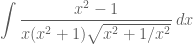
Source: I had mentioned earlier that Carl Lira had brought this integral to our attention, and he in turn had found it in the MIT Integration Bee archives. This one was from the year 1994.
Trivia: Four out of the six people who sent correct solutions are either Indians or of Indian origin! Coincidence? 🙂
Time for our next problem in the POW series! Earlier, Todd and I deliberated for a bit on whether we should pose a “hard” Ramanujan identity (involving an integral and Gamma function) as the next POW, but decided against doing it. Perhaps, we may do so some time in the future.
Okay, the following integral was brought to our attention by Carl Lira, and for the time being I won’t reveal the actual source of the problem.
Compute 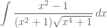
It is “hard” or “easy” depending on how you look at it!
Please send your solutions to topological[dot]musings[At]gmail[dot]com by Wednesday, June 26, 11:59pm (UTC); do not submit solutions in Comments. Everyone with a correct solution gets entered in our Hall of Fame! We look forward to your response.
The solutions are in! I thought last week’s problem might have been a little more challenging than problems of previous weeks — the identity is just gorgeous, but not at all obvious (I don’t think!) without some correspondingly gorgeous combinatorial insight. Luckily, some of our readers came up with the goods, and their solutions provide a forum for discussing a beautiful circle of ideas, involving the inter-related combinatorics of trees and endofunctions.
I can’t decide which of the solutions we received I like best. They all bear a certain familial resemblance, but each has its own distinct personality. I’ll give two representative examples, and append some comments at the end. Both proofs are conceptual “bijective” proofs, in which the two sides of the identity represent two different ways of counting essentially the same combinatorial objects. And both rely on a famous theorem of Cayley, on the number of tree structures or spanning trees on
1. (Solution by David Eppstein) As is well known (see, e.g., http://en.wikipedia.org/wiki/Pr%C3%BCfer_sequence), the number of different spanning trees on a set of n labeled nodes is 


Now suppose you are given a tree 


almost the same as the left hand side of the identity, but missing the final term in the sum.
The final term comes from the case when the marked nodes
Thus, the left side counts (partitions of n vertices into two disjoint subtrees, one subtree having one marked node and one subtree having two possibly-equal marks) + (
2. (Solution by Sune Jakobsen) Consider all 


Given a 


Using this graph, I will count the number of 


Multiplying both sides of the previous equation by and using 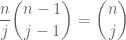 , the claim follows.
and using , the claim follows.
Remarks:
1. I found this curious identity in HAKMEM, item 118. For those who don’t know, HAKMEM is a kind of archive of cool mathematical observations made by some of the original MIT computer “hackers” from the 60’s and 70’s, including Bill Gosper and Rick Schroeppel. This particular item is credited to Schroeppel, but the accompanying text is a bit cryptic in my view:
Differentiateto get
. One observes the curious identity
(
)
and thus.
Maybe it was just their style to record a lot of their observations in such terse, compact form, but it annoys me that these guys hide their light under a bushel in this way. No motivation whatsoever, even though (I’d be willing to bet) these guys knew about the connection to trees — they’re computer scientists, after all!
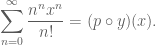
Personally, I find it easier to get from 

For, as David pointed out in his solution, 
is the exponential generating function (egf) for rooted trees.
On the other hand, it is not hard to see that the functional equation  holds for the egf of rooted trees (and uniquely determines the power series of the egf). One just applies some basic principles; I’ll just say it briefly and hope it’s somewhat followable: a rooted tree structure on a finite set is given by the selection of a root
  , together with a partition of the remainder
  into equivalence classes and a choice of rooted tree structure on each class. (Severing the root results in a bunch of disjoint subtrees, whose roots are those vertices adjacent to the original root.) At the level of egf’s, selection of the root accounts for the factor on the right of the functional equation, and if is the egf for rooted trees, then the other factor
  is the egf for the collection of ways of partitioning a set into nonempty classes and putting a rooted tree structure on each class. This is all part of the art and science of generatingfunctionology. It’s beautiful stuff.
holds for the egf of rooted trees (and uniquely determines the power series of the egf). One just applies some basic principles; I’ll just say it briefly and hope it’s somewhat followable: a rooted tree structure on a finite set is given by the selection of a root , together with a partition of the remainder into equivalence classes and a choice of rooted tree structure on each class. (Severing the root results in a bunch of disjoint subtrees, whose roots are those vertices adjacent to the original root.) At the level of egf’s, selection of the root accounts for the factor on the right of the functional equation, and if is the egf for rooted trees, then the other factor is the egf for the collection of ways of partitioning a set into nonempty classes and putting a rooted tree structure on each class. This is all part of the art and science of generatingfunctionology. It’s beautiful stuff.
Somehow I find this explanation much easier to understand than the machinations hinted at in HAKMEM 118.
2. David’s proof was actually the one I myself had in mind. I can’t say what inspired David, but I myself was inspired by an earlier reading of a beautiful (and in many respects revolutionary-for-its-time) article, on a systematic functorial approach to enumerative combinatorics:
- André Joyal, Une théorie combinatoire des séries formelles, Adv. Math. 42 (1981), 1-82.
In particular, I am very fond of the proof Joyal gives for Cayley’s theorem (which he credits to Gilbert Labelle), and this proof is in a line of thought which also leads to David’s solution. I’d like to present that proof now.
Labelle’s proof of Cayley’s theorem:
The expression 


- An equivalence relation on [
- A rooted tree structure on each equivalence class;
- A permutation structure on the set of equivalence classes (each tagged by the periodic point at the root).
Conversely, these three data determine a function, and the correspondence is bijective.
- Remark: It’s not necessary to the proof, but let me add that by basic principles of generatingfunctionology, if
], and if
is the egf for rooted trees, then
is the egf for structures given by such triplets of data. Thus, by the bijective correspondence, we have
On the other hand, consider a tree structure 

- An equivalence relation on [
- A rooted tree structure on each equivalence class;
- A spine structure (that is, a linear ordering) on the roots which tag the equivalence classes.
However, the number of linear orderings on an 
Note: regular solver Philipp Lampe, who submitted a solution similar to David’s, pointed out that there are no fewer than four proofs of Cayley’s theorem given in Aigner and Ziegler’s Proofs from The Book, which I referred to in an earlier post. At this point, I really wish I had that book! I’d be delighted if someone were to post one of those nice proofs in comments…
3. I’m not quite sure, but Sune’s solution just might be my current favorite, just because it makes obvious contact with the circle of ideas which embrace endofunctions, trees, and rooted trees (I think of the tuples there as endofunctions, or actually, partial endofunctions on
Encouraged and emboldened (embiggened?) by the ingenuity displayed by some of our readers, I’d like to see what sort of response we get to this Problem of the Week:
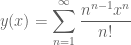
Establish the following identity:
.
(Here we make the convention
Please send your solutions to topological[dot]musings[At]gmail[dot]com by Wednesday, June 11, 11:59pm (UTC); do not submit solutions in Comments. Everyone with a correct solution gets entered in our Hall of Fame! We look forward to your response.


Recent Comments